Math Origins: Orders of Growth

When evaluating the speed of a computer program, it is useful to describe the long-run behavior of a function by comparing it to a simpler, elementary function. Today, we use many different notations to do this analysis, such as \(O\), \(o\), \(\Omega\), \(\ll\), and \(\sim\). Most of these notations express slightly different relationships between two functions, while some (like \(O\) and \(\ll\)) are equivalent.

More specifically, the \(f(x) \sim g(x)\) relation for two functions \(f, g : \mathbb{R} \to \mathbb{R}\) means that \(\displaystyle\lim_{x\to\infty}\) \(\frac{f(x)}{g(x)} = 1\). Under these conditions, the two functions are said to be asymptotically equivalent (or simply asymptotic). Alternatively, we say that \(f(x)\) is \(O(g(x))\) (pronounced "big-O of \(g(x)\)") if there are positive constants \(C\) and \(x_0\) such that \(|f(x)| \le C|g(x)|\) whenever \(x>x_0\). It is not too difficult to see that \(f(x) \sim g(x)\) implies that \(f(x)\) is \(O(g(x))\) and \(g(x)\) is \(O(f(x))\). The bigger question, though, is why there are so many different notations to express a relatively small number of concepts. The answer, as we will see, is that many different authors created and modified these ideas to suit their own purposes.  

German mathematician Paul Bachmann is credited with introducing the \(O\) notation to describe orders of magnitude in his 1894 book, Die Analytische Zahlentheorie (Analytic Number Theory). Before we explore Bachmann's work, though, it is worth remembering that mathematicians were certainly not the first to conceive of orders of magnitude in a quantitative sense. The English word order (and its cognates ordnung in German and ordre in French) derives from the Latin ordinem, which in medieval Europe was often used to describe a monastic society. Before that, it often referred to a series of ranked objects, such as threads in a loom or soldiers in a parade field.

By the 16th century, the word had been borrowed into the scientific vernacular, most notably by taxonomists who defined an order as a subgroup of a class. The basic idea was to rank or organize a set of diverse objects (for taxonomists, species; for mathematicians, functions) into classes of similar type. This use of the word was also picked up by astronomers, and began to appear in English in the 1850s. In one early example, Dionysius Lardner explained the vast distances encountered by an astronomer in his Hand-books of Natural Philosophy and Astronomy, published in 1859:

As spaces or times which are extremely great or extremely small are more difficult to conceive than those which are of the order of magnitude that most commonly falls under observation of the senses, we shall convey a more clear idea of velocity by selecting for our expression spaces and times of moderate rather than those of extreme length. The truth of this observation will be proved if we consider how much more clear a notion we have of the velocity of a runaway train, when we are told that it moves over fifteen yards per second... than when we are told that it moves over thirty miles an hour. We have a vivid and distinct idea of the length of fifteen yards, but a comparatively obscure [notion] of the length of thirty miles... [Lar, p. 75]

Since Lardner's goal was to provide an introduction to physics that could be "understood, without difficulty, by all persons of ordinary education" [Lar, p. 7], a discussion of this type is not surprising. In this excerpt, he asserted that velocities should be expressed with units of distance that are closer to everyday experience, owing to the difficulty in conceiving of orders of magnitude that are much larger or smaller than this. While modern readers may be skeptical that 30 miles per hour is harder to conceive of than 15 yards per second, we see here how orders of magnitude were used by astronomers as a quantitative concept before being adopted by Bachmann.

Paul Bachmann's Die Analytische Zahlentheorie

Returning to Bachmann's 1894 text, his overall goal was to present a full treatment of analytic number theory, which he conceived of as "investigations in the field of higher arithmetic which are based on analytical methods" [Bac, p. V]. In Chapter 13, Bachmann turned his attention to the analysis of number-theoretic functions, which included a basic theory for the number-of-divisors and sum-of-divisors functions. Today, these functions are often denoted by \(d(n)\) and \(\sigma(n)\). For example, the number \(n=6\) has the four divisors \(1\), \(2\), \(3\), and \(6\), so naturally \(d(6) = 4\) and \(\sigma(6) = 1+2+3+6 = 12\).

Of interest to us is the fact that Bachmann introduced the \(O\) notation at this point, in order to give a precise statement for the growth of the number-of-divisors function (which he denoted by \(T\)).

Figure 1. Bachmann's "big-O" notation, which appeared in his 1894 textbook, Die Analytische Zahlentheorie. Image courtesy of Archive.org.

Bachmann did not want to estimate the growth of \(T(n)\), but rather its summation function \(\sum_{k=1}^n T(k)\). So, if we wanted to compute \(\tau(6)\), we would need to compute all of \(T(1)\) through \(T(6)\), as shown in the table, resulting in \(\tau(6) = \sum_{k=1}^{6} T(k) = 14\).

Bachmann premised his argument on the fact, proven earlier in Chapter 11, that \(\tau(n)\) can be written as \(\sum_{k=1}^n \left[\frac{n}{k}\right]\), where \(\left[x\right]\) refers to the integer part of \(x\). For \(n=6\), this would result in the sum
\[
T(6) = \left[\frac{6}{1}\right]+\left[\frac{6}{2}\right]+\left[\frac{6}{3}\right]+\left[\frac{6}{4}\right]+\left[\frac{6}{5}\right]+\left[\frac{6}{6}\right] = 6+3+2+1+1+1 = 14.
\] While this is a convenient alternative formula for \(T(n)\), Bachmann wanted an analytic estimate of its magnitude—given \(n\), roughly how large is \(T(n)\)? This formula provided the starting point for his argument, which can be seen in Figure 1. First, every rational number \(x\) can be written as \(x = [x]+\{x\}\), where \(\{x\}\) is the fractional part of \(x\). As an example, the number \(x = 1.25\) can be expressed as \(x = 1 + 0.25\), where \([x] = 1\) is the integer part and \(\{x\} = 0.25\) is the fractional part. Bachmann used \(\varrho = \{x\}\) to write \(\left[\frac{n}{k}\right] = \frac{n}{k} -\varrho\). Since each of the \(n\) terms in the sum gives rise to its own \(\varrho\) and each \(\varrho\) lies between \(0\) and \(1\), we know that \(\sum_{k=1}^n \frac{n}{k}\) differs from \(\sum_{k=1}^n \left[\frac{n}{k}\right]\) by less than \(n\). As a result,
\[
\tau(n) = \sum_{k=1}^n \left[\frac{n}{k}\right] = \sum_{k=1}^n \left(\frac{n}{k} - \varrho\right) = n\cdot \sum_{k=1}^n \frac{1}{k} - r,
\] where \(r\) is the sum of the \(\varrho\)'s and is less than \(n\). He then used a formula due to Leonhard Euler,
\[
\sum_{k=1}^n \frac{1}{k} \approx E + \log n + \frac{1}{2n},
\] where \(E \approx 0.577\) is today called the Euler-Mascheroni constant. This allowed Bachmann to reach his final conclusion of \(\tau(n) = n \log n + O(n)\). These final steps are not necessarily clear, so let's take some time to work out the details. Substituting Euler's formula into the expression for \(\tau(n)\) and rearranging the terms a bit, we find that
\[
\tau(n) = n\cdot\left(E+\log n + \frac{1}{2n}\right) - r
= n\log n + \left(E\cdot n - r + \frac{1}{2}\right).
\] Focusing on the terms in the parentheses, we can see that each of \(E\cdot n\), \(r\), and \(\frac{1}{2}\) is bounded above by a constant multiple of \(n\), so their sum must also be bounded in this way. And so we arrive at Bachmann's original conclusion, that the summation function satisfies the relation \(\tau(n) = n\log n + O(n)\). Alongside his final result, Bachmann explained that the \(O(n)\) notation referred to a quantity whose order did not exceed the order of \(n\). Unfortunately, he did not clarify this definition, even though the concept was in use throughout the remainder of the book. However, it does appear that Bachmann took the notion of "order" to be self-evident at this point in time; his imprecision is not unlike Lardner's earlier use of the word.

Edmund Landau's Handbuch

Fifteen years later, Edmund Landau published his Handbuch der Lehre von der Verteilung der Primzahlen (Handbook of the Theory of the Distribution of Prime Numbers), an attempt at a complete and systematic treatment of the main results from analytic number theory. In Section 5 of his introduction, Landau used Bachmann's \(O\) notation to express a very advanced result: estimating the number of zeroes of Riemann's zeta function with imaginary part lying in the interval \((0,T]\).

Figure 2. The first appearance of "big-O" notation in Landau's Handbuch der Lehre von der Verteilung der Primzahlen (1909). Image courtesy of the University of Michigan Digital Library.

While the precise statement goes beyond the scope of the present article, we can see that Landau's definition of the \(O\) notation differs from Bachmann's. Paraphrasing slightly, by \(O(\log T)\) Landau referred to a function of \(T\) that, when divided by \(\log T\) and taken in absolute value, will remain below a fixed upper bound for all \(T\) past a certain (possibly unknown) point. This is more precise than Bachmann's definition, and gets us very close to the definition given at the beginning of this article. The only thing missing is a formalized notation for the concepts. Not one to leave the reader wanting, Landau followed up immediately with a more formal definition.

Figure 3. Landau's definition for "big-O" notation, in Handbuch der Lehre von der Verteilung der Primzahlen (1909). Image courtesy of the University of Michigan Digital Library.

Landau's final statement comes the closest to our original definition of the \(O\) notation, specifically: \(f(x)\) is \(O(g(x))\) if there exist constants \(\xi\) and \(A\) such that for all \(x\ge\xi\), \(|f(x)|<A g(x)\). In other words, \(|f(x)|\) is eventually bounded above by a constant multiple of \(g(x)\).

Landau continued more systematically in Chapter 3, at which point he developed the properties for \(O\) notation and gave definitions for both \(o\) and \(\sim\) notations.

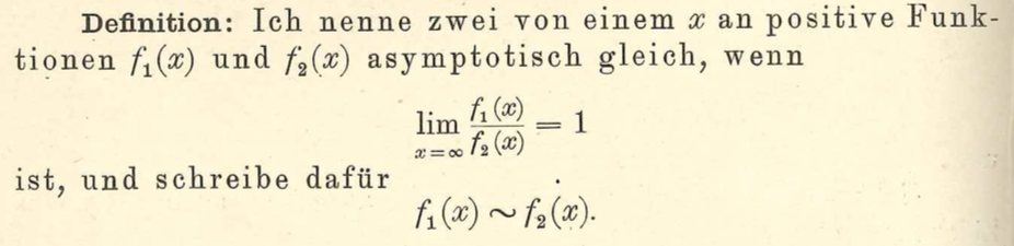
Figure 4. Landau's definitions for "little-o" and \(\sim\) notation. Images courtesy of the University of Michigan Digital Library.

While we have not yet seen the \(o\) ("little-o") notation here, both definitions conform to what we see in contemporary mathematics. It should also be noted that Landau [Lan, p. 883] gave credit to Bachmann for the \(O\) notation:

The sign \(O(g(x))\) I found first from Mr. Bachmann (1, S. 401). The \(o(g(x))\) [notation] added here corresponds to what I used to refer to in my papers with \(\{g(x)\}\).

This concludes the development for one set of notations for orders of magnitude: \(O\), \(o\), and \(\sim\). To identify the origins for some of the other notations, we follow a different historical thread that will lead us from Germany to the United Kingdom.

G. H. Hardy and Orders of Infinity: the 'Infinitärcalcül' of Paul Du Bois-Reymond

In 1877, seventeen years before Bachmann's Die Analytische Zahlentheorie appeared in print, a paper by Paul du Bois-Reymond, "Ueber die Paradoxen des Infinitärcalcüls" ("On the paradoxical infinitary calculus"), was published in Mathematische Annalen. Du Bois-Reymond was interested in providing a rigorous foundation for Calculus, and resolving the numerous apparent paradoxes that followed from the concept of infinity (especially the infinitely small). This paper was succeeded five years later by a more ambitious work, Die allgemeine Functionentheorie (The General Theory of Functions), but we can already see some new notation appearing at this early stage.

The underlying concept of the Infinitärcalcül is that of Unendlich, literally infiniteness, but more precisely the rate of increase of a function. For example, the functions \(x^2\) and \(e^x\) have different Unendlich since the rate of increase for the second function, \(e^x\), exceeds the rate of increase of the first function \(x^2\). As an example, du Bois-Reymond sought to place a bound on the size of an infinite sequence of ever-larger functions
\[
x^{1/2}, x^{2/3}, x^{3/4}, \ldots, x^{\frac{p}{p+1}}, \ldots,
\] where \(x\) is a positive real variable and \(p\) is a positive integer. Clearly, all of these exponents are bounded above by 1, so \(x\) is an example of a function whose size exceeds all of the others (at least when \(x > 1\)). However, du Bois-Reymond wanted to be more precise than this. He gave the rather complicated function \[x^\frac{\log\log x}{\log\log x\,+\,1}\] as his example for a bounding function. This function appears to come out of nowhere, but is not without its own logic. Matching the example with the general term \(x^{\frac{p}{p+1}}\), we see that du Bois-Reymond only needed to have \(p < \log\log x\) eventually, that is for sufficiently large values of \(x\), in order to reach his desired conclusion. And since \(x\) is unbounded, it is easy to see that the inequality holds as long as \(x > e^{e^p}\). So eventually, \(x^\frac{\log\log x}{\log\log x + 1}\) will exceed any particular function in the sequence. Du Bois-Reymond represented this relationship as \[x^{\frac{p}{p+1}} \prec x^\frac{\log\log x}{\log\log x + 1} \prec x,\] with the symbol \(\prec\) indicating that each function had a larger Unendlich than the one before.

Having read du Bois-Reymond's paper, and possibly also his book Die allgemeine Functionentheorie, G. H. Hardy picked up this notation and elaborated on it in his 1910 book, Orders of Infinity: the 'Infinitärcalcül' of Paul Du Bois-Reymond. This is a short book (about 60 pages in length) whose purpose was "to bring the Infinitärcalcül up to date, stating explicitly and proving carefully a number of general theorems the truth of which Du Bois-Reymond seems to have tacitly assumed..." Hardy was also interested in how orders of growth are relevant from the student's perspective, as described in his introduction.

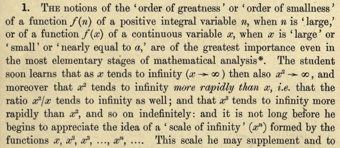
Figure 5. G. H. Hardy's motivation for studying orders of growth, from Orders of Infinity: the 'Infinitärcalcül' of Paul Du Bois-Reymond (1910). Image courtesy of Archive.org.

Hardy's goal, then, was to refine Du Bois-Reymond's notion of Unendlich to benefit students of analysis. True to his word, Hardy followed on his initial comments with a comprehensive set of definitions to clarify his notion of "order of greatness," as seen below.

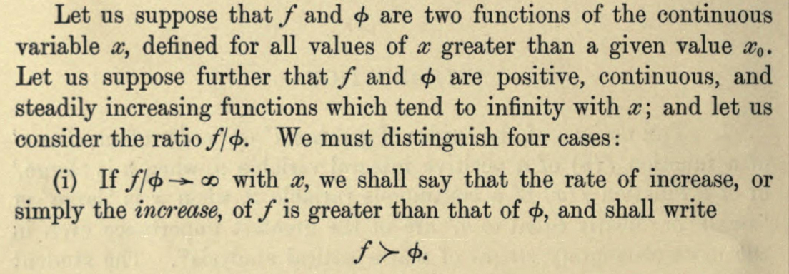
Figure 6. Hardy's use of \(\succ\), \(\prec\), and \(\asymp\) notations, from Orders of Infinity: the 'Infinitärcalcül' of Paul Du Bois-Reymond (1910). Images courtesy of Archive.org.

Clearly, the \(\prec\) notation was borrowed from Du Bois-Reymond, though today it is not typically used to compare orders of growth. Hardy also used \(\asymp\) instead of the more modern "big Theta" notation \(\Theta\), which was promoted by Donald Knuth [Knu] in the 1970s. However, we do continue to use the \(\sim\) notation (apparently borrowed from Landau) to indicate that the limit of ratios is equal to 1.

Hardy's next step was to establish a set of basic properties that would allow a student to easily assess and compare orders of growth.

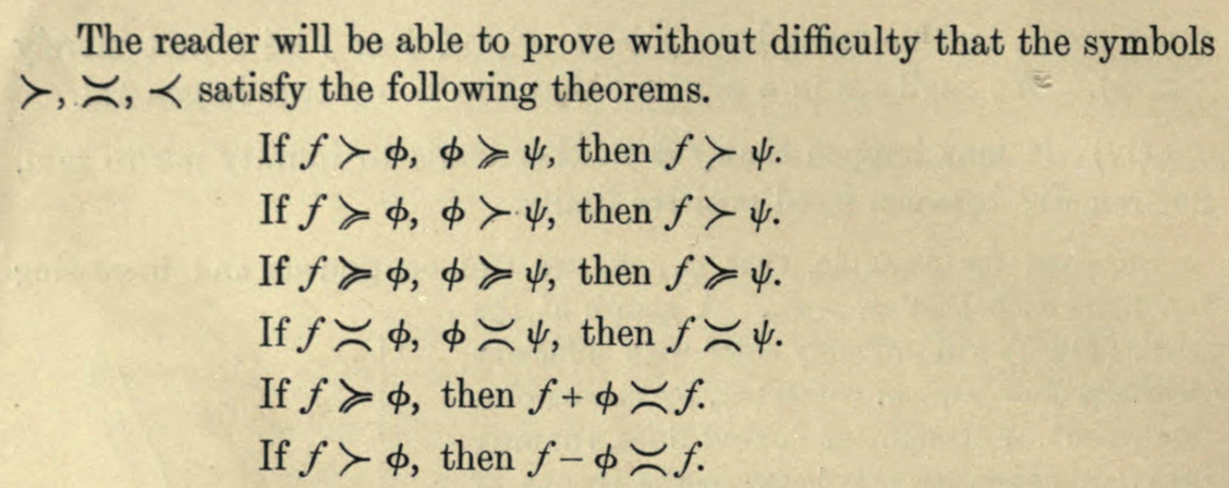
Figure 7. Elementary results about Hardy's asymptotic notations in Orders of Infinity: the 'Infinitärcalcül' of Paul Du Bois-Reymond (1910). Images courtesy of Archive.org.

Having left these proofs to the reader, Hardy then turned to Landau's \(O\) notation.

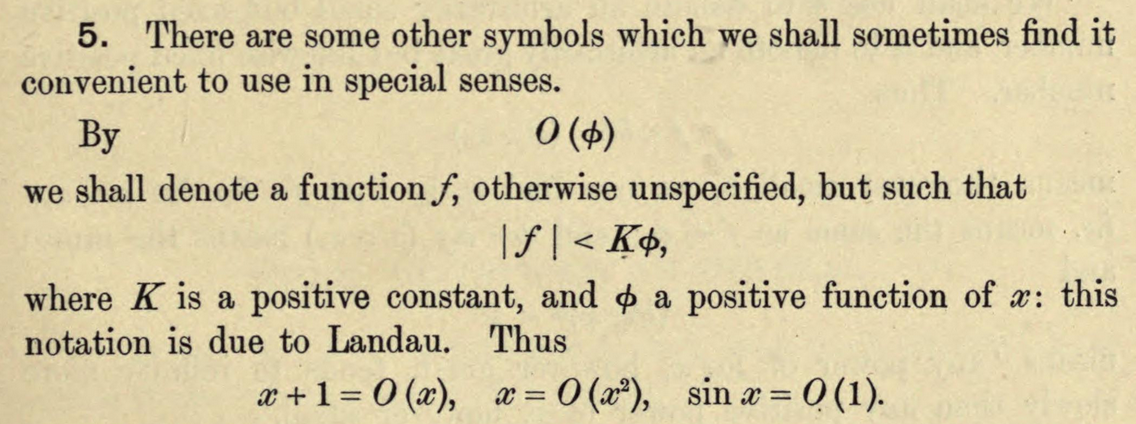
Figure 8. Hardy's definition for "big-O" notation in Orders of Infinity: the 'Infinitärcalcül' of Paul Du Bois-Reymond (1910). Interestingly, Hardy gave credit to Landau, though Bachmann had used the notation several years earlier. Image courtesy of Archive.org.

It is interesting that, in spite of his clear desire to develop a comprehensive set of notations to describe orders of growth, Hardy still introduced the big-O notation here. Looking back to his definition for \(\asymp\), we can see that using \(O\) is equivalent to using only the upper bound in \(\asymp\). Clearly, he was familiar with Landau's work and felt the notation was either useful or common enough to merit inclusion here. It also appears that he was unaware that Landau himself borrowed the big-O notation from Bachmann.

One may wonder justifiably why, given that previous notations existed, Hardy chose to attempt this revision at all. Indeed, one early review of Orders of Infinity addressed this exact issue. In his review of the book for the Bulletin of the American Mathematical Society [Hur], W. A. Hurwitz wrote:

One is impelled to wonder how much of the fairly extensive notation introduced will be found really desirable in actual use of the results. The notations of inferior and superior limit have won a permanent place; Landau's symbols \(O(f)\) and \(o(f)\) have in a short time come into such wide use as apparently to insure their retention. It is doubtful whether any further notation will be found necessary.

As is often the case, a notational choice can quickly become entrenched, and potential improvements are often cast aside in favor of a familiar—if inelegant—system. One final note here: twenty-four years later, Ivan Vinogradov [Vin] used the notation \(f(x) \ll g(x)\) as yet another alternative to writing \(f(x) = O(g(x))\). Unlike some of Hardy's symbols, this one continues to be used today.

Conclusion

So, while the notations for orders of growth were originally developed by analytic number theorists in the late 19th century, they came to be used by analysts in the early 20th century, and were adopted by computer scientists in the late 20th century. Moreover, the differing choices of these individuals led to a several different ways of expressing similar ideas. For example, we know that the expressions \(f(x) = O(g(x))\) and \(f(x) \ll g(x)\) have the same meaning, with the \(\ll\) having been introduced by Landau in 1909 and Vinogradov in 1934, respectively. Additionally, the expressions \(f(x) = \Theta(g(x))\) and \(f(x) \asymp g(x)\) have the same meaning, though the former was due to Hardy in 1910, while the latter came into use due to Knuth in the 1970s. While Landau's "big-O" notation was adopted early, the varied interests of scholars gave space for redundant or nuanced terms to be defined as circumstances dictated. Undoubtedly, not all mathematics is developed in a clean and concise way, and here we see that the path to new mathematical truths can be a meandering one.

References

[Bac] Bachmann, Paul. Die analytische Zahlentheorie. Leipzig: Teubner, 1894.

[duB] du Bois-Reymond, Paul. "Ueber die Paradoxen des Infinitärcalcüls." Math. Ann. (June 1877) 11, Issue 2, 149-167.

[Har] Hardy, G. H. Orders of Infinity: the "Infinitärcalcül" of Paul Du Bois-Reymond. Cambridge University Press, 1910.

[Hur] Hurwitz, Wallie A. Review: G. H. Hardy, Orders of Infinity. The "Infinitärcalcül" of Paul Du Bois-Reymond. Bull. Amer. Math. Soc. 21, No. 4 (1915), 201-202.

[Knu] Knuth, Donald. "Big Omicron and Big Theta and Big Omega." SIGACT News (April-June 1976) 8, Issue 2, 18-24.

[Lan] Landau, Edmund. Handbuch der Lehre von der Verteilung der Primzahlen. Leipzig: Teubner, 1909.

[Lar] Larder, Dionysius. Hand-books of Natural Philosophy and Astronomy. Philadelphia: Blanchard and Lea, 1859.

[Vin] I. M. Vinogradov. "A new estimate for \(G(n)\) in Waring's problem" Dokl. Akad. Nauk SSSR 5 (1934), 249–253.