A Selection of Problems from A.A. Markov’s Calculus of Probabilities: Problem 4 – A Simple Gambling Game
This is an example of what would later be called a Markov chain. It has a two-dimensional state space of the form \((x, y)\), where \(x\) is the fortune of player \(L\) and \(y\) is the fortune of player \(M\). States \((l, 0), (l, 1), \dots, (l, m - 1)\) and \((0, m), (1, m), \dots, (l - 1, m)\), are absorbing, meaning that once the chain enters one of these states, it cannot leave. The only transitions are from state \((x, y)\) to state \((x + 1, y)\), with probability \(p\), and to state \((x, y + 1)\), with probability \(q\), except when \((x, y)\) is absorbing. Ironically, when Markov started writing about experiments connected in a chain in 1906, his examples were nothing like this one.12 Even in the fourth edition of the book, which was published 18 years after he first wrote about chains, he still used the same approach as he did here.
Problems of this type were studied by Pierre-Simon Laplace (1749–1827), Daniel Bernoulli (1700–1782), and Viktor Bunyakovskiy (1804–1889), among others, long before Markov. However, these works were almost certainly not the motivation for Markov's development of chains.
|
Задача 4ая. Два игрока, которых мы назовём \(L\) и \(M\), играют в некоторую игру, состоящую из последовательных партий. Каждая отдельная партия должна окончиться для одного из двух игроков \(L\) и \(M\) выигрышем её, а для другого проигрышем, при чем вероятность выиграть её для \(L\) равна \(p\), а для \(M\) равна \(q=1-p\), независимо от результатов других партий. Вся игра окончиться, когда \(L\) выиграет \(l\) партий или \(M\) выиграет \(m\) партий: в первом случае игру выиграет \(L\), а в втором \(M\). Требуется опреледить вероятности выиграть игру для игрока \(L\) и для игрока \(M\), которые мы обозначим символами \((L)\) и \((M)\). Эта задача известна с половины семнадцатого столетия и заслуживает особого внимания, так как в различных приёмах, предположенных Паскалем и Ферматом для её решения, можно видеть начало исчисления вероятностей. |
4th Problem. Two players, whom we call \(L\) and \(M\), play a certain game consisting of consecutive rounds.
Each individual round must end by one of the two players \(L\) and \(M\) winning it and the other losing it, where the probability of winning for \(L\) is \(p\) and for \(M\) is \(q = 1 - p\), independent of the results of the other rounds.
The entire game is finished when \(L\) wins \(l\) rounds or \(M\) wins \(m\) rounds. In the first case, the game is won by \(L\), and in the second, by \(M\).
It is required to determine the probabilities of winning the game for player \(L\) and player \(M\), which we denote by the symbols \(L\) and \(M\).
This problem has been known since the middle of the 17th century and deserves particular attention, since distinct methods of solution proposed by Pascal and Fermat can be seen as the beginning of the calculus of probabilities.
Continue to Markov's first solution of Problem 4.
Skip to Markov's second solution of Problem 4.
Skip to Markov's numerical example for Problem 4.
Skip to statement of Problem 8.
[12] In Markov's papers on chains, he restricted himself to chains with two states. His primary example was to consider the alternation between vowels and consonants in Alexander Pushkin's novel-in-verse, Eugene Onegin. Specifically, he wanted to determine if it is more likely for a vowel to be followed by a consonant or by another vowel. See [Hayes 2013] for more information on this work.
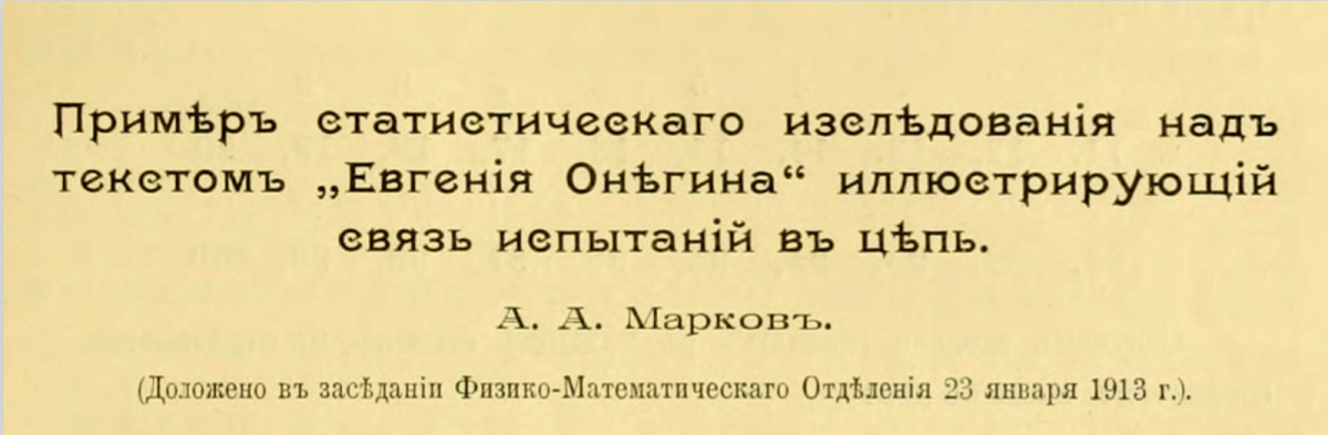
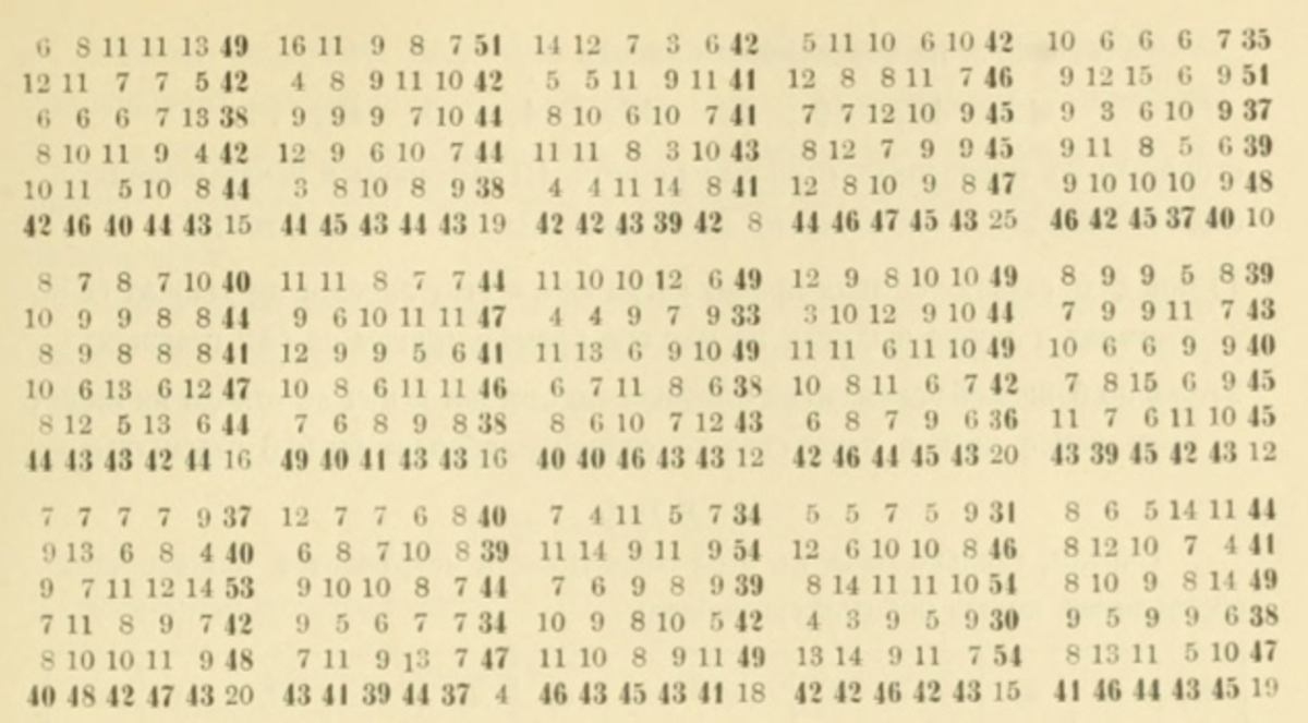
Figure 6. The title and part of Markov’s analysis of the frequency of vowels and consonants in
Eugene Onegin. Slides for “First Links of the Markov Chain: Probability and Poetry,” by Brian Hayes, 23 January 2013.
A Selection of Problems from A.A. Markov’s Calculus of Probabilities: Problem 4 – Solution 1
Review statement of Problem 4.
Solution 1: First of all, we note that the game can be won by player \(L\) in various numbers of rounds not less than \(l\) and not more than \(l + m - 1\).
Therefore, by the Theorem of Addition of Probabilities,13 we can represent the desired probability \((L)\) in the form of a sum \((L)_l + (L)_{l+1} + \cdots + (L)_{l+i} + \cdots + (L)_{l+m-1}\), where \((L)_{l+i}\) denotes the total probability that the game is finished in \(l+i\) rounds won by player \(L\).
And in order for the game to be won by player \(L\) in \(l+i\) rounds, that player must win the \((l+i)\)th round and must win exactly \(l-1\) of the previous \(l+i-1\) rounds.
Hence, by the Theorem of Multiplication of Probabilities,14 the value of \((L)_{l+i}\) must be equal to the product of the probability that player \(L\) wins the \((l+i)\)th round and the probability that player L wins exactly \(l-1\) out of \(l+i-1\) rounds.
The last probability, of course, coincides with the probability that in \(l+i-1\) independent experiments, an event whose probability for each experiment is \(p\), will appear exactly \(l-1\) times.
The probability that player \(L\) wins the \((l+i)\)th round is equal to \(p\), as is the probability of winning any round.
Then15 \[(L)_{l+i} = p \frac{1\cdot 2\cdot \cdots\cdot (l+i-1)}{1\cdot 2\cdot \cdots\cdot i \cdot 1\cdot 2\cdot \cdots\cdot (l-1)} p^{l-1} q^i = \frac{l (l+1)\cdot \cdots\cdot (l+i-1)}{1\cdot 2\cdot \cdots\cdot i} p^l q^i,\] and finally, \[(L) = p^l\left\lbrace 1 + \frac{l}{1}q + \frac{l(l+1)}{1\cdot 2}q^2 + \cdots + \frac{l(l+1)\cdots(l+m-2)}{1\cdot 2\cdot \cdots\cdot(m-1)} q^{m-1}\right\rbrace.\]
In a similar way, we find \[(M) = q^m\left\lbrace 1 + \frac{m}{1}p + \frac{m(m+1)}{1\cdot 2}p^2 + \cdots + \frac{m(m+1)\cdots(m+l-2)}{1\cdot 2\cdot \cdots\cdot(l-1)} p^{l-1}\right\rbrace.\]
However, it is sufficient to calculate one of these quantities, since the sum \((L)+ (M)\) must reduce to 1.
Continue to Markov's second solution of Problem 4.
Skip to Markov's numerical example for Problem 4.
Skip to statement of Problem 8.
[13] This “theorem,” presented in Chapter I, says (in modern notation): If \(A\) and \(B\) are disjoint, then \(P(A \cup B) = P(A) + P(B)\). We would now consider this an axiom of probability theory. Since Markov considered only experiments with finite, equiprobable sample spaces, he could “prove” this by a simple counting argument.
[14] This “theorem,” also presented in Chapter I, says (in modern notation): \(P(A \cap B) = P(A |B) \cdot P(B)\). Nowadays, we would consider this as a definition of conditional probability, a term Markov never used. Again, he “proved” it using a simple counting argument. He then defined the concept of independent events.
[15] The conclusion \((L)_{l+i} = \binom{l+i-1}{i}p^l q^i\) is a variation of the negative binomial distribution; namely, if \(X\) represents the number of Bernoulli trials needed to attain \(r\) successes, then \(P(X=n) = \binom{n-1}{r-1}p^r q^{n-r},\ \ n\geq r\), where \(p\) is the probability of success on each trial and \(q=1-p\).
A Selection of Problems from A.A. Markov’s Calculus of Probabilities: Problem 4 – Solution 2
Review statement of Problem 4.
Solution 2: Noting that the game must end in no more than \(l+m-1\) rounds, we assume that a player does not stop immediately upon achieving one of the appropriate numbers of winning rounds but continues to play until exactly \(l+m-1\) rounds are played.
Under these assumptions, the probability that player \(L\) wins the game is equal to the probability of winning, by that same player \(L\), no fewer than \(l\) rounds out of all \(l+m-1\) rounds.
In this case, if the game is won by player \(L\), then the number of rounds won by him reaches the value \(l\) and the subsequent rounds can only increase this number, or leave it unchanged.
And conversely, if player \(L\) wins no fewer than \(l\) rounds out of \(l+m-1\) rounds, then the number of rounds won by player \(M\) will be less than \(m\); hence, in that case, it follows that player \(L\) wins \(l\) rounds before player \(M\) manages to win \(m\) rounds and, in this way, the game will be won by player \(L\).
On the other hand, the probability that player \(L\) wins no fewer than \(l\) rounds out of \(l+m-1\) rounds coincides with the probability that, in \(l+m-1\) independent experiments, an event whose probability for each experiment is \(p\) appears no fewer than \(l\) times.
The previous probability is expressed by the known sum of products \[\frac{1\cdot 2\cdot \cdots\cdot (l+m-1)}{1\cdot 2\cdot \cdots\cdot (l+i) \cdot 1\cdot 2\cdot \cdots\cdot (m-i+1)} p^{l+i} q^{m-i+1}\]
where \(i= 0,1,2,\dots,m-1\).
Then \[(L) = \frac{(l+m-1)\cdot\cdots\cdot m}{1\cdot2 \cdot\cdots\cdot l} p^l q^{m-1} \left\lbrace 1 + \frac{m-1}{l+1} \frac{p}{q} + \frac{m-1}{l+1}\frac{m-2}{l+2}\frac{p^2}{q^2} + \cdots \right\rbrace;\] also, we find \[(M) = \frac{(l+m-1)\cdot\cdots\cdot l}{1\cdot2 \cdot\cdots\cdot m} p^{l-1} q^{m} \left\lbrace 1 + \frac{l-1}{m+1}\frac{q}{p} + \frac{l-1}{m+1} \frac{l-2}{m+2} \frac{q^2}{p^2} + \cdots \right\rbrace.\]
It is not hard to see that these new expressions for \((L)\) and \((M)\) are equal to those found previously.16
Continue to Markov's numerical example for Problem 4.
Skip to statement of Problem 8.
[16] Note that the second solution demonstrates a nice connection between the binomial and negative binomial distributions. This argument is essentially the following theorem: If \(Y\) has a binomial distribution with parameters \(n\) and \(p\), and \(T\) has a negative binomial distribution with parameters \(r\) and \(p\), where \(n\geq r\), then \(P(Y \geq r) = P(T \leq n)\). In other words, if it takes no more than \(n\) trials to get \(r\) successes (\(T \leq n\)), then there must have been at least \(r\) successes in the first \(n\) trials (\(Y \geq r\)).
A Selection of Problems from A.A. Markov’s Calculus of Probabilities: Problem 4 – Numerical Examples
Review statement of Problem 4.
Numerical examples:
\(\mathrm{1)}\ \ p = q = \dfrac{1}{2},\ l=1,\ m=2\).
\[ \begin{align} (L) &= p(1+q) = 2pq\left(1+ \dfrac{1}{2}\dfrac{p}{q}\right) = \dfrac{3}{4}, \\
(M) &= q^2 = \dfrac{1}{4}. \end{align} \]
\(\mathrm{2)}\ \ p=\dfrac{2}{5},\ q= \dfrac{3}{5},\ l=2,\ m=3\).
\[ \begin{align} (L) &= p^2\left\lbrace 1+ 2q + 3q^2\right\rbrace = 6p^2q^2\left\lbrace1 + \dfrac{2}{3}\dfrac{p}{q} + \dfrac{1}{6}\dfrac{p^2}{q^2}\right\rbrace = \dfrac{328}{625}. \\ (M) &= q^3 \left\lbrace 1+ 3p \right\rbrace = 4q^3 p\left\lbrace 1 + \dfrac{1}{4}\dfrac{q}{p}\right\rbrace = \dfrac{297}{625}. \end{align} \]
Continue to Markov's statement of Problem 8.