A Selection of Problems from A.A. Markov’s Calculus of Probabilities
In 1900, Andrei Andreevich Markov (1856–1922) wrote the first edition of the book, Calculus of Probabilities (Исчисление Вероятностей). This was around the time that Russian mathematicians became interested in probability, so this book was likely one of the first comprehensive Russian texts on the subject. Three more editions followed—in 1908, 1912, and, posthumously, 1924. Parts of the second and third editions have been translated into French and German, but there appears to be no English translation of any of the editions until now.
In this article, I present an English translation of five of the eight problems, and worked solutions, from Chapter IV of the first edition of Markov’s book (Problems 1, 2, 3, 4, and 8). With some updating of notation and terminology, these could have been written today and, thus, are particularly amenable for discussion in elementary probability courses. In particular, these examples (and all other examples in the first four chapters) have finite, equiprobable sample spaces. In addition, after presenting the five worked problems, I include some additional analysis provided by Markov on calculating probabilities of repeated independent events, using what today we would label as Bernoulli random variables.
It is generally agreed that the origin of the formal study of probability dates to the 17th century, when mathematicians such as Blaise Pascal (1623–1662), Pierre de Fermat (1601–1665), and Jakob Bernoulli (1655–1705) were interested in games of chance.1 As we see, that focus continues here with these problems from Markov’s book. Problems 5, 6 and 7 of Chapter IV are simply variations on Problem 4.
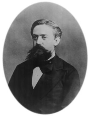
Figure 1. A. A. Markov (1856–1922).
Convergence Portrait Gallery.
In what follows, I begin with some biographical information about Markov followed by further details about the various editions and translations of his book. I then present the English translations of the five selected problems, with some brief commentary on each. I close by offering some specific suggestions about how instructors could use the translated material with students in various elementary probability courses.
Readers may navigate this article either by using the table of contents listed at the bottom of this page, or by using the hierarchical outline provided here:
- Biographical information about A. A. Markov
- Brief history of his book, Calculus of Probabilities
- Presenting the problems
- Problem 1: Selecting balls from a vessel
- Problem 2: A lottery game
- Problem 3: Some generalizations of Problem 2
- Problem 4: A simple gambling game
- Problem 8: Sums of independent random variables
- Calculating probabilities of repeated independent events
- Suggestions for the classroom and conclusion
Readers interested in my full translation of Markov’s first edition may find it here.
[1] One place to begin exploring the early history of probability is the 2015 Convergence article, “The ‘Problem of Points’ and Perseverance,” by Keith Devlin.
A Selection of Problems from A.A. Markov’s Calculus of Probabilities: Andrei Andreevich Markov
Andrei Andreevich Markov was born on June 14, 1856, in Ryazan Gubernia (governorate, similar to a state in the US) in Russia, the son of Andrei Grigorevich Markov, a successful lawyer. He graduated from the gymnasium (high school) in 1874 and enrolled in Petersburg University, where he received a gold medal for his work, On Integration of Differential Equations with the Help of Continued Fractions.
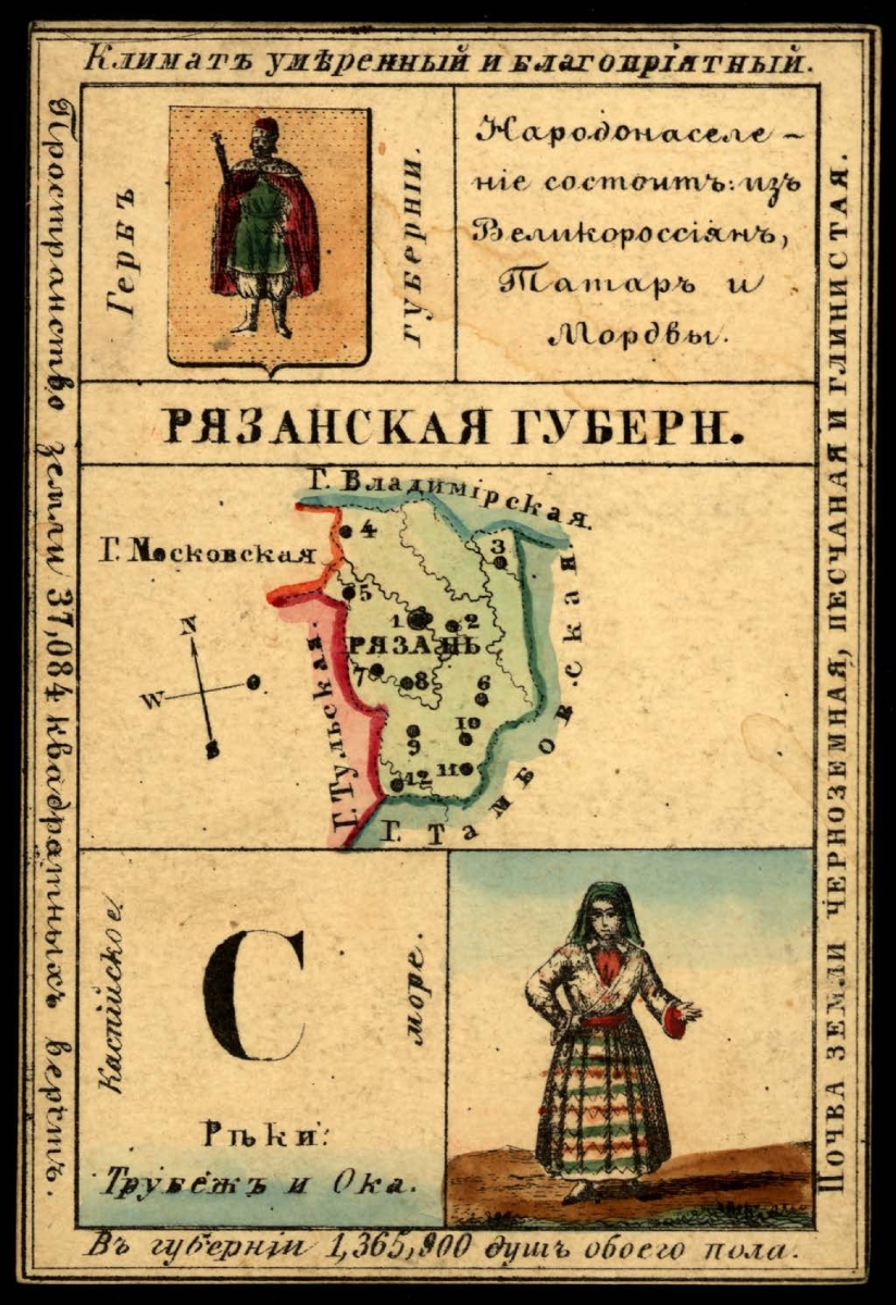
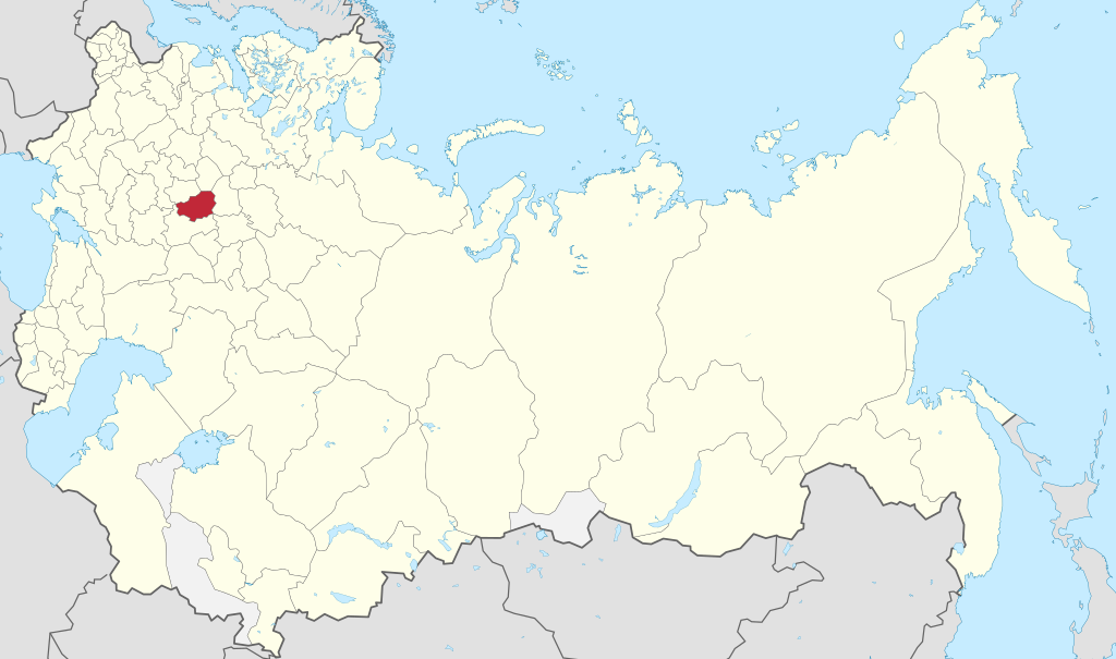
Figure 2. A card from a geographical card set with a map of Ryazan Gubernia in 1856
and the governorate located within the Russian Empire as it existed in 1914.
Wikimedia Commons, public domain and created by Milenioscuro, CC BY-SA 4.0 DEED.
He defended his master’s degree dissertation, On Binary Quadratic Forms with Positive Determinant, in 1880, under the supervision of Aleksandr Korkin (1837–1908) and Yegor Zolotarev (1847–1878). He then wrote his doctoral dissertation, On Some Applications of Algebraic Continued Fractions, under the supervision of Pafnuty Lvovich Chebyshev (1821–1894), in 1884. Markov taught at Petersburg University until 1905, but he continued to conduct research there until his death from sepsis after an operation on his leg on July 20, 1922.
Markov married Maria Ivanova Valvatyeva in 1883. They had one son, also named Andrei Andreevich Markov (1903–1979), who became a mathematician, noted for his work in constructive mathematics and logic. In 1951, the younger Andrei wrote a book, Selected Works (Избранные Труды), containing some of his father’s contributions to mathematics.
At some point in the 1890s, Markov became interested in probability, especially limiting theorems of probabilities, laws of large numbers and least squares (which is related to his work on quadratic forms). One point of emphasis was on generalizations of the Central Limit Theorem, where he eventually weakened the independence requirement, replacing it with dependence of each variable only on its immediate predecessor. This ultimately led to his work on what would be known later as Markov chains in 1906.2 Specifically, a Markov chain is a discrete-state stochastic process \(\{X_1,X_2,X_3,\ldots,\}\) in which the probability mass function of \(X_n\) depends only on the value of \(X_{n-1}\) and not on the values of any previous variables; that is, \(P(X_n=j|X_{n-1}=i, X_{n-2}, X_{n-3},\ldots)=P(X_n=j|X_{n-1}=i)=p_{ij}\). The first use of the term “Markov chain” was most likely by Sergei N. Bernstein (1880–1968) in [Bernstein 1927].
[2] For more information on the development of Markov chains, see [Basharin et al. 2004] and [Seneta 1996].
A Selection of Problems from A.A. Markov’s Calculus of Probabilities: Markov's Book
Figure 3. Title page of the first edition. GoogleBooks.
As noted in the overview, the four editions of Markov's Calculus of Probabilities appeared in 1900, 1908, 1912, and, posthumously, 1924. Parts of the second and third editions have been translated into French and German, but there appears to have been no English translation of any of the editions until now. The first edition (from 1900) contains eight chapters.3
| Pages | ||
|---|---|---|
| Chapter I | Basic concepts and theorems | 1–20 |
| Chapter II | On repeated experiments | 21–51 |
| Chapter III | On the sum of independent variables | 52–100 |
| Chapter IV | Examples of various methods of calculating probabilities | 101–157 |
| Chapter V | Limits, irrational numbers and continuous variables in the calculus of probabilities | 158–187 |
| Chapter VI | Probability of hypotheses and future events | 188–212 |
| Chapter VII | The method of least squares | 213–266 |
| Chapter VIII | On life insurance | 267–279 |
The fourth edition (of 1924) is approximately twice the length of the first edition. Much of the extra material is in Chapter VII, which tripled in size. There is some additional material—which he could have called “chapters”—on limit theorems, method of moments, and experiments connected in a chain. Since this edition was published after Markov's death, it contains a biographical sketch of Markov written by his student, Abram Bezicovich (1891–1970). I have included that sketch in my full translation of the first edition (pp. 9–17).
[3] A translation of the entire first edition can be found at: https://digital.fandm.edu/calculusofprobabilities.
About the translation, it is fair to say that Russian does not translate smoothly into English. Russian word order is quite flexible and punctuation rules are different. The lack of the present tense of the verb “to be” leads to excessive use of passive voice. I have tried to translate the work as literally as possible, within the bounds of sensible English.
The original Russian first edition of the text can be found at this link. The Russian language was simplified a bit after the Russian Revolution in 1917. Some letters were removed from the alphabet and there were some spelling changes. Most notably, the “hard sign”, ъ, (твёрдый знак), which appeared at the end of many words that ended in a consonant, was eliminated (although it can still be found in the middle of some words). The fourth edition incorporates many of these modifications. I have retyped the first edition in the modern Russian language. It is available upon request.
A Selection of Problems from A.A. Markov’s Calculus of Probabilities: Presenting the Problems
My translations of Markov's statements of the five selected problems are given on the following pages.
- Problem 1: Selecting balls from a vessel
- Problem 2: A lottery game
- Problem 3: Some generalizations of Problem 2
- Problem 4: A simple gambling game
- Problem 8: Sums of independent random variables
As a preface to each problem statement, I provide a few comments (in italics) at the top of the associated page. The original Russian statement of the problem is then given, followed by its English translation.
Links to my translation of Markov's solution for each problem are provided at the bottom of the associated statement page; my own commentaries on Markov's work appear either in footnotes or in italicized text on the solution pages.
Following my translation of the solution of Problem 8, I also provide my translation of Markov's analysis of the binomial distribution (as we would now call it) on the following three pages which should be read sequentially:
- Calculating probabilities of repeated independent events, Part 1
- Calculating probabilities of repeated independent events, Part 2
- Calculating probabilities of repeated independent events, Part 3
A Selection of Problems from A.A. Markov’s Calculus of Probabilities: Problem 1 – Selecting Balls from a Vessel
This problem is very elementary and can be found in nearly every modern probability textbook, where it might be phrased as “selection without replacement.” It is a standard hypergeometric distribution example.
|
Задача 1ая. Из сосуда, содержащего \(a\) белых и \(b\) чёрных шаров и никаких других, вынимают одновременно или последовательно \(\alpha+\beta\) шаров, при чем, в случае последовательного вынимания, ни один из вынутых шаров не возвращают обратно в сосуд и новых туда также не подкладывают. Требуется определить вероятность, что между вынутыми таким образом шарами будеть \(\alpha\) белых и \(\beta\) чёрных. |
1st Problem. From a vessel containing \(a\) white and \(b\) black balls and no others, we select, simultaneously or consecutively, \(\alpha + \beta\) balls, for which, in the case of consecutive selection, none of the chosen balls are returned to the vessel and new ones are also not put back in.
It is required to determine the probability that there will be \( \alpha \) white and \(\beta \) black among the balls selected in this way.
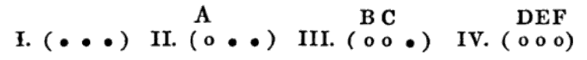
Figure 4. Augustus De Morgan’s illustration of a ball and vessel problem with three balls,
from page 53 of his 1838 Essay on Probabilities. Convergence Mathematical Treasures.
Continue to Markov's solution of Problem 1.
Skip to statement of Problem 2.
A Selection of Problems from A.A. Markov’s Calculus of Probabilities: Problem 1 – Solution
Review statement of Problem 1.
Solution: Assume that all the balls in the vessel are distinguished from one another by numbers in such a way that the white balls have numbers \(1, 2, 3, \dots, a\) and the black have numbers \(a+1, a+2, \dots, a+b\).
The numbers on the chosen balls must form some set of \(\alpha + \beta\) numbers from all \(a+b\) numbers \(1, 2, 3, \dots, a+b\).
The number of different sets of \(\alpha + \beta\) numbers that can be formed from \(a+b\) numbers is equal to \[\frac{(a+b)(a+b-1)(a+b-2)\cdots (a + b - \alpha - \beta +1)}{1\cdot 2 \cdot 3 \cdot\cdots \cdot (\alpha + \beta)}.\]
Corresponding to this, we can distinguish \[\frac{(a+b)(a+b-1)(a+b - 2) \cdots (a+b - \alpha - \beta +1)}{1\cdot 2 \cdot 3 \cdot\cdots \cdot (\alpha + \beta)}\] equally likely cases, each of which consists of the appearance of a specific \(\alpha + \beta\) numbers.
From all these exhaustive and disjoint cases, the appearance of \(\alpha\) white and \(\beta\) black balls is favored only for those in which any set of \(\alpha\) numbers from the group \(1, 2, 3,\dots, a\), together with any \(\beta\) numbers from the group \(a+1, a+2, \dots, a+b\), appear.
The number of distinct sets of \(\alpha\) numbers that can be formed from \(a\) numbers is equal to \(\frac{a(a-1) \cdots (a- \alpha + 1)}{1\cdot 2\cdot\cdots \cdot \alpha}\) and the number of distinct sets of \(\beta\) numbers that can be formed from \(b\) numbers is equal to \(\frac{b(b-1) \cdots (b- \beta + 1)}{1\cdot 2\cdot\cdots \cdot \beta}\).
Therefore, the number of distinct sets of \(\alpha + \beta\) numbers that can be formed from \(a+b\) numbers is expressed by the product \[ \frac{a(a-1) \cdots (a- \alpha + 1)}{1\cdot 2\cdot\cdots \cdot \alpha} \cdot \frac{b(b-1) \cdots (b- \beta + 1)}{1\cdot 2\cdot\cdots \cdot \beta}.\]
Then the number of cases considered that favor the appearance of \(\alpha\) white and \(\beta\) black balls is expressed by the indicated product.
And, consequently, the desired probability that among the chosen \(\alpha + \beta\) balls, there will be \(\alpha\) white and \(\beta\) black is expressed by the ratio \[\frac{\frac{a(a-1) \cdots (a- \alpha + 1)}{1\cdot 2\cdot\cdots \cdot \alpha} \cdot \frac{b(b-1) \cdots (b- \beta + 1)}{1\cdot 2\cdot\cdots \cdot \beta}} {\frac{(a+b)(a+b-1)(a+b-2)\cdots (a + b - \alpha - \beta +1)}{1\cdot 2 \cdot 3 \cdot\cdots \cdot (\alpha + \beta)}},\] which, after simple transformations, reduces to4 \[\frac{1\cdot 2 \cdot 3 \cdot\cdots \cdot (\alpha + \beta)}{1\cdot 2 \cdot\cdots \cdot \alpha \cdot 1\cdot 2 \cdot\cdots \cdot \beta} \cdot \frac{a(a-1) \cdots(a- \alpha + 1) \cdot b(b-1) \cdots (b- \beta + 1)}{(a+b)(a+b - 1)(a+b - 2) \cdots (a + b - \alpha - \beta +1)}.\]
Continue to Markov's presentation of a numerical example for Problem 1.
Skip to statement of Problem 2.
[4] In more compact notation, the solution reduces to: \(\frac{\binom{a}{\alpha} \binom{b}{\beta}}{\binom{a+b}{\alpha+\beta}}\).
A Selection of Problems from A.A. Markov’s Calculus of Probabilities: Problem 1 – Numerical Example
Review statement of Problem 1.
\(a=3,\ b=4,\ \alpha =2,\ \beta= 2 \).
Let us assume the white balls are set by the numbers 1, 2, 3 and the black by the numbers 4, 5, 6, 7.
The numbers on the chosen four balls can be represented by any of the following \(\frac{7 \cdot 6 \cdot 5 \cdot 4}{1\cdot 2 \cdot 3 \cdot4} = 35 \) sets:
| 1, 2, 3, 4 | 1, 2, 3, 5 | 1, 2, 3, 6 | 1, 2, 3, 7 | 1, 2, 4, 5 | 1, 2, 4, 6 | 1, 2, 4, 7 |
| 1, 2, 5, 6 | 1, 2, 5, 7 | 1, 2, 6, 7 | 1, 3, 4, 5 | 1, 3, 4, 6 | 1, 3, 4, 7 | 1, 3, 5, 6 |
| 1, 3, 5, 7 | 1, 3, 6, 7 | 1, 4, 5, 6 | 1, 4, 5, 7 | 1, 4, 6, 7 | 1, 5, 6, 7 | 2, 3, 4, 5 |
| 2, 3, 4, 6 | 2, 3, 4, 7 | 2, 3, 5, 6 | 2, 3, 5, 7 | 2, 3, 6, 7 | 2, 4, 5, 6 | 2, 4, 5, 7 |
| 2, 4, 6, 7 | 2, 5, 6, 7 | 3, 4, 5, 6 | 3, 4, 5, 7 | 3, 4, 6, 7 | 3, 5, 6, 7 | 4, 5, 6, 7 |
If two white and two black balls are chosen, then their numbers form one of the following \(\frac{3\cdot 2}{1\cdot2} \times \frac{4\cdot3}{1\cdot2} = 18\) sets:
| 1, 2, 4, 5 | 1, 2, 4, 6 | 1, 2, 4, 7 | 1, 2, 5, 6 | 1, 2, 5, 7 | 1, 2, 6, 7 |
| 1, 3, 4, 5 | 1, 3, 4, 6 | 1, 3, 4, 7 | 1, 3, 5, 6 | 1, 3, 5, 7 | 1, 3, 6, 7 |
| 2, 3, 4, 5 | 2, 3, 4, 6 | 2, 3, 4, 7 | 2, 3, 5, 6 | 2, 3, 5, 7 | 2, 3, 6, 7 |
In this way, we have 35 equally likely cases, 18 of which favor the considered event; consequently, the desired probability that there will be two of each color among the four chosen balls is \(\frac{18}{35}\).5
Note that Markov did not use “\(!\)” for factorial or any combinatorial notation such as \(\binom{n}{k}\) or \(\,_n C_k\), although such symbols had been around since the early 19th century. There are many other places in the text where Markov's writing could be simplified if even more modern terminology, such as “sample space,” “normal distribution,” and “variance” had been invented.
Markov provided a second solution to this problem. It is rather convoluted and not much is gained by including it here. It can be found (together with another numerical example) in the complete translation (pp. 78–80).
[5] In other words, \( \frac{\binom{3}{2}\binom{4}{2}}{\binom{7}{4}} = \frac{18}{35} \).
A Selection of Problems from A.A. Markov’s Calculus of Probabilities: Problem 2 – A Lottery Game
This problem is similar to the first, but Markov included an application to a lottery game dating back to 17th-century France. Games of chance were the primary motivation for some of the early writings on probability by Fermat, Pascal, Huygens, and others. Lotteries of this type are found today in many states in the US. It would be interesting to compare the probabilities and payoffs in current games to the ones mentioned here.
|
Задача 2ая. Из сосуда, содержащего \(n\) билетов с нумерами \(1, 2, 3, \dots, n\) и никаких других, вынимают одновременно или последовательно m билетов, при чем, в сдучае последовательного вынимания, ни один из вынутых билетов не возвращают обратно в сосуд и новых туда также не покладывают. Требуется определить вероятность, что между нумерами вынутых билетов появятся \(i\) нумеров, указанных заранее, напр. \(1, 2, 3, \dots, i\). |
2nd Problem. From a vessel containing \(n\) tickets with numbers \(1, 2, 3, \dots, n\), and no others, we select, simultaneously or consecutively, \(m\) tickets, so that in the case of consecutive selection, none of the selected tickets is returned to the vessel and a new one is removed.
It is required to find the probability that, among the numbers on the chosen tickets, \(i\) numbers, indicated in advance, appear—for example, \(1, 2, 3, \dots, i\).
Continue to Markov's solution of Problem 2.
Skip to statement of Problem 3.
A Selection of Problems from A.A. Markov’s Calculus of Probabilities: Problem 2 – Solution
Review statement of Problem 2.
Solution: This problem can be considered as a special case of the previous, with \(a = \alpha\).
Namely, there are \(i\) tickets, whose numbers are chosen in advance, that are similar to the white balls, and the remaining tickets are similar to the black balls.
This similarity immediately reveals that the solution to the posed problem is obtained from the previous through substituting all numbers \(a,\, b,\, \alpha,\, \beta\) by the corresponding numbers \(i,\, n-i,\, i,\, m-i\).
Returning on that basis to the expression \[\frac{1\cdot 2 \cdot 3 \cdot\cdots \cdot (\alpha + \beta)}{1\cdot 2 \cdot\cdots \cdot \alpha \cdot 1\cdot 2 \cdot\cdots \cdot \beta} \cdot \frac{a(a-1) \cdots(a- \alpha + 1) \cdot b(b-1) \cdots (b- \beta + 1)}{(a+b)(a+b - 1) \cdots (a + b - \alpha - \beta +1)}\] found earlier, and making the indicated substitutions, we find the value of the desired probability in the form of the product \[\frac{1\cdot 2 \cdot 3 \cdot\cdots \cdot m}{1\cdot 2 \cdot\cdots \cdot i \cdot 1\cdot 2 \cdot\cdots \cdot (m-i)} \, \frac{i(i-1) \cdots 1 \cdot (n-i)(n-i-1) \cdots (n-m + 1)}{n(n - 1) \cdots (n-m +1)}\] which, after cancellation, reduces to6 \[ \frac{m (m-1) \cdots (m-i+1)}{n(n-1) \cdots (n-i+1)}.\]
Thus, the desired probability that among the chosen \(m\) numbers all of the \(i\) numbers indicated in advance appear is expressed by the fraction \[\frac{m (m-1) \cdots (m-i+1)}{n(n-1) \cdots (n-i+1)}.\]
Here, as with the first problem, Markov includes a second solution, which we omit.
Continue to an application of Problem 2.
Skip to statement of Problem 3.
[6] In modern notation, this becomes \(\frac{\binom{a}{\alpha} \binom{b}{\beta}}{\binom{a+b}{\alpha+\beta}} = \frac{\binom{n-i}{m-i}}{\binom{n}{m}}\), which is equivalent to the stated answer.
A Selection of Problems from A.A. Markov’s Calculus of Probabilities: Problem 2 – An Application to a Contemporary Lottery
Review statement of Problem 2.
For example, let us turn our attention to a lottery which, in the past, was played in France and many regions of Germany.7
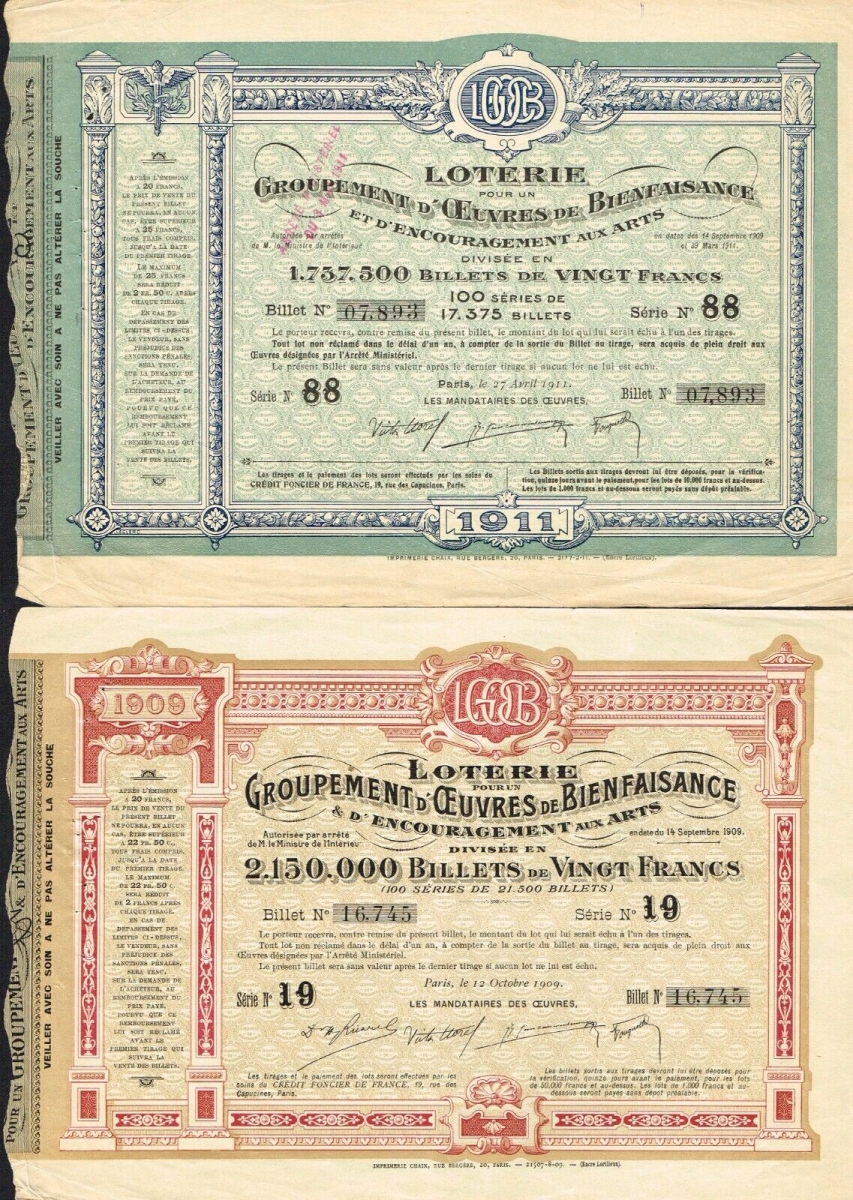
Figure 5. Two billettes from French lotteries, one dated 27 April 1911 (upper image),
the other 12 October 1909 (lower image). Offered for auction at eBay, September–October 2023.
It consists of 90 numbers and, in each drawing, five numbers appeared. By the rules of the lottery, it was possible to place one or another amount on any numbers, or on any set of two, three, four or, finally, five numbers, which were called, respectively, l'extrait simple, l'ambe, le terne, le quaterne, and le quine.
If the five published numbers were found in the set on which the player placed an amount, then the administrator of the lottery gave an agreed-upon sum, found by a specific ratio to the amount of the bet, to that player.
These ratios are:
for l'extrait simple............................................................................................................ 15,
for l'ambe....................................................................................................................... 270,
for le terne.................................................................................................................... 5500,
for le quaterne........................................................................................................... 75 000,
for le quine............................................................................................................ 1 000 000.
In order to calculate the probabilities that l'extrait simple, l'ambe, le terne, le quaterne, and le quine appear, we should set \(n = 90\) and \(m = 5\) in the expression \(\frac{m (m-1) \cdots (m-i+1)}{n(n-1) \cdots (n-i+1)}\) we found, and give \(i\) the values \(1, 2, 3, 4, 5\), consecutively.
In this way, we find that the probability of the appearance of
l'extrait simple is equal to ................................................................................... \(\dfrac{5}{90} = \dfrac{1}{18}\),
l'ambe......................................................................................................... \(\dfrac{5 \cdot 4}{90 \cdot 89} = \dfrac{2}{801}\),
le terne........................................................................................... \(\dfrac{5 \cdot 4 \cdot 3}{90 \cdot 89 \cdot 88} = \dfrac{1}{11\,748}\),
le quaterne .......................................................................... \(\dfrac{5 \cdot 4 \cdot 3 \cdot 2}{90 \cdot 89 \cdot 88 \cdot 87} = \dfrac{1}{511\,038}\),
le quine................................................................................ \(\dfrac{1}{511\,038} \cdot\dfrac{1}{86} = \dfrac{1}{43\,949\,268}\).
Therefore, if the player's bet is \(M\), then the mathematical expectation8 of his profit from participating in the lottery
is expressed by:
in the case of l'extrait simple........................................................... \(\left(\frac{15}{18} - 1\right) M = -\frac{1}{6} M\),
in the case of l'ambe.................................................................... \(\left(\frac{540}{801} -1\right) M = -\frac{29}{89}M\),
in the case of le terne........................................................... \(\left(\frac{5500}{11\,748} - 1 \right)M = -\frac{1562}{2987}M\),
and so on.
In all cases, as we see, the mathematical expectation is a negative number; consequently, the lottery in question represented a game that was far from harmless.
This result corresponds to the fact that the lottery yielded a significant profit for its organizers.
Continue to statement of Problem 3.
[7] One of the earliest such lotteries was the Génoise Lottery in France in the early 17th century. It was used there and in other countries to replenish government treasuries. See [Maistrov 1974], and the references contained therein, for more information.
[8] The Russian term “математическое ожидание” translates as “mathematical expectation.” It is more common to say “expected value” in modern terminology.
A Selection of Problems from A.A. Markov’s Calculus of Probabilities: Problem 3 – Some Generalizations of Problem 2
This problem contains five generalizations of the previous problem. The first two are fairly straightforward, but later solutions become increasingly complex. Markov makes some interesting approximations involving Taylor series. There are ample opportunities for the reader to fill in details.
|
Задача 3ья. Из сосуда, содержащего \(n\) билетов с нумерами \(1, 2, 3, \dots, n\) и никаких других, вынимают одновременно \(m\) билетов, что мы назовём первым тиражем. Затем вынутые билеты возвращают в сосуд и производят подобный же второй тираж m билетов. По окончании второго тиража вынутые билеты возвращают также в сосуд и производят третий тираж \(m\) билетов и т.д. Требуется при \(k\) таких тиражах определить: 1) вероятность, что \(i\) определённых нумеров не появятся; 2) вероятность, что \(i\) определённых нумеров не появятся, а другие \(l\) определённых нумеров появятся; 3) вероятность, что \(l\) определённых нумеров появятся; 4) вероятность, что появятся только \(l\) определённых нумеров; 5) вероятность, что появятся все нумера. |
3rd Problem. From a vessel containing \(n\) tickets with numbers \(1, 2, 3, \dots, n\), and no others, we select simultaneously \(m\) tickets, which we call the first draw.
Then the chosen tickets are returned to the vessel and we produce a similar second draw of \(m\) tickets. Upon finishing the second draw, the chosen tickets are again returned to the vessel and we produce a third draw of \(m\) tickets, etc.
It is required to determine, for \(k\) such draws:
1) the probability that \(i\) specific numbers do not appear;
2) the probability that \(i\) specific numbers do not appear, but another \(l\) specific numbers do appear;
3) the probability that \(l\) specific numbers appear;
4) the probability that only \(l\) specific numbers appear;
5) the probability that all numbers appear.
Continue to Markov's solution of Problem 3, Parts 1 and 2.
Continue to Markov's solution of Problem 3, Parts 3, 4, and 5.
Skip to statement of Problem 4.
A Selection of Problems from A.A. Markov’s Calculus of Probabilities: Problem 3 – Solution to Parts 1 and 2
Review statement of Problem 3.
Solution: For brevity, let \[\left\lbrace \frac{p(p-1) \cdots (p-m+1)}{1\cdot2\cdot\cdots\cdot m}\right\rbrace^k = Z_p ,\] for any number \(p\).
On each draw, the number of selected tickets can represent any set of \(m\) numbers from all \(n\) numbers \(1, 2, \dots, n\).
Corresponding to this, on one draw we distinguish \(\frac{n(n-1)\cdots(n-m+1)}{1\cdot2\cdot\cdots\cdot m}\) equally likely cases, and on \(k\) draws, we distinguish \(\left\lbrace \frac{n(n-1)\cdots(n-m+1)}{1\cdot2\cdot\cdots\cdot m}\right \rbrace^k = Z_n\) equally likely cases.9
Each of the preceding exhaustive and disjoint cases consists of the appearance of \(k\) specific sets of \(m\) numbers on the \(k\) draws considered.
Establishing in this way those cases that we will consider, and showing the total number of them, we proceed to determine the probabilities of the events referred to in the problem by calculating the number of cases favorable to them.
If \(i\) specific numbers \(\alpha_1, \alpha_2, \dots, \alpha_i\) do not appear, then for one draw, instead of \(\frac{n(n-1)\cdots(n-m+1)}{1\cdot2\cdot\cdots\cdot m}\), there remain \(\frac{(n-i)(n-i-1)\cdots(n-i-m+1)}{1\cdot2\cdot\cdots\cdot m}\) cases, and for \(k\) draws, we have \(\left\lbrace\frac{(n-i)(n-i-1)\cdots(n-i-m+1)}{1\cdot2\cdot\cdots\cdot m}\right\rbrace^k = Z_{n-i}\) cases, instead of \(\left\lbrace \frac{n(n-1)\cdots(n-m+1)}{1\cdot2\cdot\cdots\cdot m}\right \rbrace^k = Z_n\).
Thus, the probability that, for the \(k\) draws considered, \(i\) specific numbers do not appear is given by the fraction \[\frac{Z_{n-i}}{Z_n} = \left\lbrace\frac{(n-i)(n-i-1)\cdots(n-i-m+1)}{n(n-1)\cdots(n-m+1)}\right\rbrace^k.\]
Then the number of cases for which the \(i\) specific numbers \(\alpha_1, \alpha_2, \dots, \alpha_i\) do not appear and one specific number \(\beta_1\) does appear can be expressed by the difference \(\Delta Z_{n-i-1} = Z_{n-i} - Z_{n-i-1}\), where according to what we just said, \(Z_{n-i}\) represents the number of cases in which the numbers \(\alpha_1, \alpha_2, \dots, \alpha_i\) do not appear, and \(Z_{n-i-1}\) the number of those cases in which, besides the numbers \(\alpha_1, \alpha_2, \dots, \alpha_i\), the number \(\beta_1\) also does not appear.
In a similar manner, the number of cases in which the numbers \(\alpha_1, \alpha_2, \dots, \alpha_i\) do not appear and two specific numbers do appear can be expressed by the second difference \(\Delta^2 Z_{n-i-2} = \Delta Z_{n-i-1} - \Delta Z_{n-i-2}\), where \(\Delta Z_{n-i-1}\) represents the number of all cases in which the number \(\beta_1\) does appear and the numbers \(\alpha_1, \alpha_2, \dots, \alpha_i\) do not appear, and \(\Delta Z_{n-i-2}\) the number of those cases in which, besides \(\alpha_1, \alpha_2, \dots, \alpha_i\), the number \(\beta_2\) also does not appear.
In view of the possibility of continuing similar reasoning, it is not difficult to conclude that, in general, the number of cases in which \(i\) specific numbers do not appear and another \(l\) specific numbers do appear can be represented by the \(l\)th order difference \(\Delta^l Z_{n-i-l}\), which is equal to: \[Z_{n-i} - \frac{l}{1}Z_{n-i-1} + \frac{l(l-1)}{1\cdot2} Z_{n-i-2} - \cdots \pm Z_{n-i-l}.\]
Then the probability that, in the \(k\) draws considered, \(i\) specific numbers do not appear and another \(l\) specific numbers do appear is equal to10 \[\frac{\Delta^l Z_{n-i-l}}{Z_n}.\]
Continue to Markov's solution of Problem 3, Parts 3, 4, and 5.
Skip to statement of Problem 4.
[9] In other words, \(Z_p = \binom{p}{m}^k\) for any \(p\), so that \(Z_n = \binom{n}{m}^k\).
[10] For example, suppose \(n = 10, m = 3,\) and \(k = 5\). The total number of outcomes is \(Z_{10}=\binom{10}{3}^5=120^5\). For question (1), let \(i = 2\), so that we consider the number of selections without two numbers \(\alpha_1\) and \(\alpha_2\) in any of the 5 draws. There are \(Z_8=\binom{8}{3}^5=56^5\) such selections. Hence, the probability that \(\alpha_1\) and \(\alpha_2\) do not appear is \(\frac{Z_8}{Z_{10}}=\frac{56^5}{120^5} \approx 0.02213\). For question (2), the number of selections without \(\alpha_1\) and \(\alpha_2\) and containing another number \(\beta_1\) is: \[\Delta Z_7 = Z_8 - Z_7 = \binom{8}{3}^5-\binom{7}{3}^5 = 498~209~901.\] Of these, \[\Delta Z_6 = Z_7 - Z_6 = \binom{7}{3}^5 - \binom{6}{3}^5 = 49~321~875\] do not contain some other number \(\beta_2\). So, the number of selections without \(\alpha_1\) and \(\alpha_2\) and containing \(\beta_1\) and \(\beta_2\) is: \[\Delta^2 Z_6 = \Delta Z_7 - \Delta Z_6 = Z_8 - 2 Z_7 + Z_6 = 448~888~026,\] and the probability of this event is \(\frac{\Delta^2 Z_6}{Z_{10}} = \frac{448~888~026}{120^5} \approx 0.01804\). Similarly, \(\frac{\Delta^3 Z_5}{Z_{10}} = \frac{Z_8 - 3Z_7 + 3Z_6 - Z_5}{120^5} \approx 0.01618\).
A Selection of Problems from A.A. Markov’s Calculus of Probabilities: Problem 3 – Solution to Parts 3, 4 and 5
Review statement of Problem 3.
The other probabilities referred to in the problem represent three particular cases of the probability just found and, therefore, can be gotten from the expression \(\frac{\Delta^l Z_{n-i-l}}{Z_n}\) for particular assumptions about \(i\) and \(l\): \[\mathrm{1)}\ i=0, \ \ \ \ \mathrm{2)}\ i=n-l,\ \ \ \ \mathrm{3)}\ i=0, l=n.\]
Letting \(i = 0\), we get the following expression for the probability of the appearance of \(l\) specific numbers: \[\frac{\Delta^l Z_{n-l}}{Z_n} = 1 - \frac{l}{1}\left(\frac{n-m}{n}\right)^k + \frac{l(l-1)}{1\cdot2} \left(\frac{n-m}{n}\right)^k \left(\frac{n-m-1}{n-1}\right)^k - \cdots \]
Letting \(i = n - l\), we find that the probability of the appearance of \(l\) specific numbers and the nonappearance of the remaining is equal to:
\[\begin{align} \frac{\Delta^l Z_0}{Z_n} &= \frac{Z_l}{Z_n} - \frac{l}{1}\frac{Z_{l-1}}{Z_n} + \frac{l(l-1)}{1 \cdot 2} \frac{Z_{l-2}}{Z_n} - \cdots \\ &= \left(\frac{n-m}{n}\right)^k \left(\frac{n-m-1}{n-1}\right)^k \cdots \left(\frac{l-m+1}{l+1}\right)^k \left\lbrace 1 - \frac{l}{1} \left(\frac{l-m}{l}\right)^k + \cdots \right\rbrace. \end{align}\]
Finally, the probability of the appearance of all \(n\) numbers is equal to:
\[\frac{\Delta^n Z_0}{Z_n} = 1 - \frac{n}{1}\left(\frac{n-m}{n}\right)^k + \frac{n(n-1)}{1\cdot2} \left(\frac{n-m}{n}\right)^k \left(\frac{n-m-1}{n-1}\right)^k - \cdots.\]
Stopping at the last formula and noting that it requires tedious calculation for large values of \(n\), we derive two approximate formulas for it.
For getting the first approximate formula, assume that all numbers \(\left(\frac{n-m-1}{n-1}\right)^k\), \(\left(\frac{n-m-2}{n-2}\right)^k, \dots\), are equal to \(\left(\frac{n-m}{n}\right)^k\) which, for brevity, we denote by the letter \(t\).
Under this assumption, the indicated formula immediately gives us: \[\frac{\Delta^n Z_0}{Z_n} \approx (1-t)^n,\] where \(t = \left(\frac{n-m}{n}\right)^k\).
For the second approximation, we note that for small values of \(i\), the ratio \(\left(\frac{n-m-i}{n-i}\right)^k : \left(\frac{n-m}{n}\right)^k \), which is equal to \(\left\lbrace 1 - \frac{im}{(n-i)(n-m)}\right\rbrace^k\), differs little from \(1 - \frac{kim}{n(n-m)}\), and the product \[\left(1 - \frac{km}{n(n-m)} \right) \left(1 - \frac{2km}{n(n-m)} \right) \cdots \left(1 - \frac{ikm}{n(n-m)} \right) \] differs little from \[1-\frac{km(1+2+\cdots+i)}{n(n-m)} = 1 - \frac{kmi(i+1)}{2n(n-m)}.\]
On this basis, we accept \(t^{i+1}\left(1 - \frac{kmi(i+1)}{2n(n-m)}\right)\) as the approximate value of each product \[\left(\frac{n-m}{n}\right)^k \left(\frac{n-m-1}{n-1}\right)^k \cdots \left(\frac{n-m-i}{n-i}\right)^k.\]
Substituting this approximate expression in place of the exact one in the formula, we get \[\frac{\Delta^n Z_0}{Z_n} \approx (1-t)^n - \frac{kmt^2(n-1)}{2(n-m)}(1-t)^{n-2}\approx (1-t)^n\left\lbrace1-\frac{kmt^2}{2}\right\rbrace,\] since we assume the numbers \(\frac{n-1}{n-m}\) and \(\frac{1}{(1-t)^2}\) are close to 1.
We apply our approximate formula to finding the number of draws under the hypothesis that the probability of the appearance of all numbers was approximately equal to a given number \(\frac{1}{C}\).
The first approximation formula gives \((1-t)^n \approx \frac{1}{C}\) from which we deduce \(n \log(1-t) \approx -nt \approx -\log C\); but \(t = \left(\frac{n-m}{n}\right)^k\) and, thus, \(\log t = k \log\left(1- \frac{m}{n}\right) \approx - \frac{km}{n}\).11
Comparing the approximate equations \(-nt \approx -\log C\) and \(\log t \approx -\frac{km}{n}\), we find \[k \approx \frac{n(\log n- \log \log C)}{m} .\]
In the subsequent calculation, let \(\frac{\log C}{n} = t_0\) and \(\frac{n(\log n- \log \log C)}{m} = k_0\), so that \(t_0\) and \(k_0\) are the approximate values of the numbers \(t\) and \(k\).
The second approximate expression of the probability gives \((1-t)^n \left(1-\frac{kmt^2}{2}\right) \approx \frac{1}{C}\), from which, by performing the approximate calculations, we deduce
\[\log C \approx nt + \frac{nt^2}{2} + \frac{kmt^2}{2} \approx nt + \frac{(n+k_0 m) t_0^2}{2},\]
\[t \approx \frac{\log C}{n} \left[ 1-\frac{(n+k_0 m)t_0^2}{2 \log C}\right],\]
and then \[-\log t \approx \log n- \log \log C + \frac{(n + k_0 m) t_0^2}{2 \log C}.\]
On the other hand, we have \[ -\log t = -k \log\left(1-\frac{k}{m}\right) \approx \frac{km}{n} + \frac{k_0 m^2}{2n^2}.\]
Finally, equating one approximate expression for $\log t$ to the other, we arrive at the approximate equation \[ \frac{km}{n} + \frac{k_0 m^2}{2n^2} \approx \log n - \log \log C + \frac{(n + k_0 m) t_0^2}{2 \log C},\] from which we easily deduce
\[\begin{align} k &\approx \frac{n}{m} \left\lbrace \log n - \log \log C + \frac{k_0 m}{2 n^2}(\log C - m) + \frac{1}{2n} \log C\right\rbrace \\
&\approx \frac{1}{m} \left\lbrace (\log n - \log \log C) \left( n + \frac{1}{2} \log C - \frac{m}{2} \right) + \frac{1}{2} \log C\right\rbrace.
\end{align}\]
For example, let us assume \(n= 90,\ m=5,\ C=2\).
Then
| \(\log n = 4.4998\dots\), | \(\log C = 0.69314\dots\), |
| \(\log \log C = -0.3665\dots\), | \(n + \frac{1}{2} \log C - \frac{m}{2} = 87.84657\dots\). |
and, performing a simple calculation by the previous approximate formula, we get \[k = \frac{4.8663 \times 87.8466 + 0.346}{5} \approx 85.5.\]
According to this result, it can be verified that the probability of the appearance of all 90 numbers in 85 draws is somewhat less than one-half, and for 86 draws is already bigger than one-half.
Continue to statement of Problem 4.
[11] Here, Markov used “log” to denote natural (base \(e\)) logarithms. Later, he used the same notation for common (base 10) logarithms!
The Taylor series for \(\ln(1-t)\) is \(-t -\frac{t^2}{2} - \frac{t^3}{3} - \cdots \approx -t\), for small values of t. (The series converges for \(-1 \leq t < 1\).) Later, he included the quadratic term for a better approximation.
A Selection of Problems from A.A. Markov’s Calculus of Probabilities: Problem 4 – A Simple Gambling Game
This is an example of what would later be called a Markov chain. It has a two-dimensional state space of the form \((x, y)\), where \(x\) is the fortune of player \(L\) and \(y\) is the fortune of player \(M\). States \((l, 0), (l, 1), \dots, (l, m - 1)\) and \((0, m), (1, m), \dots, (l - 1, m)\), are absorbing, meaning that once the chain enters one of these states, it cannot leave. The only transitions are from state \((x, y)\) to state \((x + 1, y)\), with probability \(p\), and to state \((x, y + 1)\), with probability \(q\), except when \((x, y)\) is absorbing. Ironically, when Markov started writing about experiments connected in a chain in 1906, his examples were nothing like this one.12 Even in the fourth edition of the book, which was published 18 years after he first wrote about chains, he still used the same approach as he did here.
Problems of this type were studied by Pierre-Simon Laplace (1749–1827), Daniel Bernoulli (1700–1782), and Viktor Bunyakovskiy (1804–1889), among others, long before Markov. However, these works were almost certainly not the motivation for Markov's development of chains.
|
Задача 4ая. Два игрока, которых мы назовём \(L\) и \(M\), играют в некоторую игру, состоящую из последовательных партий. Каждая отдельная партия должна окончиться для одного из двух игроков \(L\) и \(M\) выигрышем её, а для другого проигрышем, при чем вероятность выиграть её для \(L\) равна \(p\), а для \(M\) равна \(q=1-p\), независимо от результатов других партий. Вся игра окончиться, когда \(L\) выиграет \(l\) партий или \(M\) выиграет \(m\) партий: в первом случае игру выиграет \(L\), а в втором \(M\). Требуется опреледить вероятности выиграть игру для игрока \(L\) и для игрока \(M\), которые мы обозначим символами \((L)\) и \((M)\). Эта задача известна с половины семнадцатого столетия и заслуживает особого внимания, так как в различных приёмах, предположенных Паскалем и Ферматом для её решения, можно видеть начало исчисления вероятностей. |
4th Problem. Two players, whom we call \(L\) and \(M\), play a certain game consisting of consecutive rounds.
Each individual round must end by one of the two players \(L\) and \(M\) winning it and the other losing it, where the probability of winning for \(L\) is \(p\) and for \(M\) is \(q = 1 - p\), independent of the results of the other rounds.
The entire game is finished when \(L\) wins \(l\) rounds or \(M\) wins \(m\) rounds. In the first case, the game is won by \(L\), and in the second, by \(M\).
It is required to determine the probabilities of winning the game for player \(L\) and player \(M\), which we denote by the symbols \(L\) and \(M\).
This problem has been known since the middle of the 17th century and deserves particular attention, since distinct methods of solution proposed by Pascal and Fermat can be seen as the beginning of the calculus of probabilities.
Continue to Markov's first solution of Problem 4.
Skip to Markov's second solution of Problem 4.
Skip to Markov's numerical example for Problem 4.
Skip to statement of Problem 8.
[12] In Markov's papers on chains, he restricted himself to chains with two states. His primary example was to consider the alternation between vowels and consonants in Alexander Pushkin's novel-in-verse, Eugene Onegin. Specifically, he wanted to determine if it is more likely for a vowel to be followed by a consonant or by another vowel. See [Hayes 2013] for more information on this work.
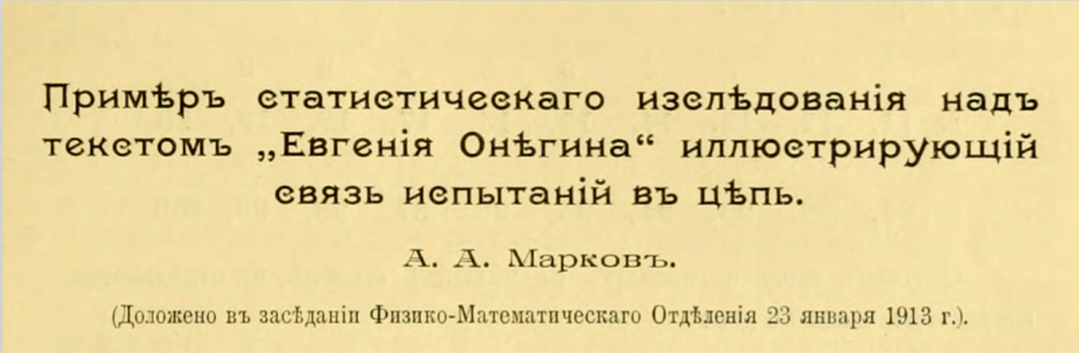
Figure 6. The title and part of Markov’s analysis of the frequency of vowels and consonants in
Eugene Onegin. Slides for “First Links of the Markov Chain: Probability and Poetry,” by Brian Hayes, 23 January 2013.
A Selection of Problems from A.A. Markov’s Calculus of Probabilities: Problem 4 – Solution 1
Review statement of Problem 4.
Solution 1: First of all, we note that the game can be won by player \(L\) in various numbers of rounds not less than \(l\) and not more than \(l + m - 1\).
Therefore, by the Theorem of Addition of Probabilities,13 we can represent the desired probability \((L)\) in the form of a sum \((L)_l + (L)_{l+1} + \cdots + (L)_{l+i} + \cdots + (L)_{l+m-1}\), where \((L)_{l+i}\) denotes the total probability that the game is finished in \(l+i\) rounds won by player \(L\).
And in order for the game to be won by player \(L\) in \(l+i\) rounds, that player must win the \((l+i)\)th round and must win exactly \(l-1\) of the previous \(l+i-1\) rounds.
Hence, by the Theorem of Multiplication of Probabilities,14 the value of \((L)_{l+i}\) must be equal to the product of the probability that player \(L\) wins the \((l+i)\)th round and the probability that player L wins exactly \(l-1\) out of \(l+i-1\) rounds.
The last probability, of course, coincides with the probability that in \(l+i-1\) independent experiments, an event whose probability for each experiment is \(p\), will appear exactly \(l-1\) times.
The probability that player \(L\) wins the \((l+i)\)th round is equal to \(p\), as is the probability of winning any round.
Then15 \[(L)_{l+i} = p \frac{1\cdot 2\cdot \cdots\cdot (l+i-1)}{1\cdot 2\cdot \cdots\cdot i \cdot 1\cdot 2\cdot \cdots\cdot (l-1)} p^{l-1} q^i = \frac{l (l+1)\cdot \cdots\cdot (l+i-1)}{1\cdot 2\cdot \cdots\cdot i} p^l q^i,\] and finally, \[(L) = p^l\left\lbrace 1 + \frac{l}{1}q + \frac{l(l+1)}{1\cdot 2}q^2 + \cdots + \frac{l(l+1)\cdots(l+m-2)}{1\cdot 2\cdot \cdots\cdot(m-1)} q^{m-1}\right\rbrace.\]
In a similar way, we find \[(M) = q^m\left\lbrace 1 + \frac{m}{1}p + \frac{m(m+1)}{1\cdot 2}p^2 + \cdots + \frac{m(m+1)\cdots(m+l-2)}{1\cdot 2\cdot \cdots\cdot(l-1)} p^{l-1}\right\rbrace.\]
However, it is sufficient to calculate one of these quantities, since the sum \((L)+ (M)\) must reduce to 1.
Continue to Markov's second solution of Problem 4.
Skip to Markov's numerical example for Problem 4.
Skip to statement of Problem 8.
[13] This “theorem,” presented in Chapter I, says (in modern notation): If \(A\) and \(B\) are disjoint, then \(P(A \cup B) = P(A) + P(B)\). We would now consider this an axiom of probability theory. Since Markov considered only experiments with finite, equiprobable sample spaces, he could “prove” this by a simple counting argument.
[14] This “theorem,” also presented in Chapter I, says (in modern notation): \(P(A \cap B) = P(A |B) \cdot P(B)\). Nowadays, we would consider this as a definition of conditional probability, a term Markov never used. Again, he “proved” it using a simple counting argument. He then defined the concept of independent events.
[15] The conclusion \((L)_{l+i} = \binom{l+i-1}{i}p^l q^i\) is a variation of the negative binomial distribution; namely, if \(X\) represents the number of Bernoulli trials needed to attain \(r\) successes, then \(P(X=n) = \binom{n-1}{r-1}p^r q^{n-r},\ \ n\geq r\), where \(p\) is the probability of success on each trial and \(q=1-p\).
A Selection of Problems from A.A. Markov’s Calculus of Probabilities: Problem 4 – Solution 2
Review statement of Problem 4.
Solution 2: Noting that the game must end in no more than \(l+m-1\) rounds, we assume that a player does not stop immediately upon achieving one of the appropriate numbers of winning rounds but continues to play until exactly \(l+m-1\) rounds are played.
Under these assumptions, the probability that player \(L\) wins the game is equal to the probability of winning, by that same player \(L\), no fewer than \(l\) rounds out of all \(l+m-1\) rounds.
In this case, if the game is won by player \(L\), then the number of rounds won by him reaches the value \(l\) and the subsequent rounds can only increase this number, or leave it unchanged.
And conversely, if player \(L\) wins no fewer than \(l\) rounds out of \(l+m-1\) rounds, then the number of rounds won by player \(M\) will be less than \(m\); hence, in that case, it follows that player \(L\) wins \(l\) rounds before player \(M\) manages to win \(m\) rounds and, in this way, the game will be won by player \(L\).
On the other hand, the probability that player \(L\) wins no fewer than \(l\) rounds out of \(l+m-1\) rounds coincides with the probability that, in \(l+m-1\) independent experiments, an event whose probability for each experiment is \(p\) appears no fewer than \(l\) times.
The previous probability is expressed by the known sum of products \[\frac{1\cdot 2\cdot \cdots\cdot (l+m-1)}{1\cdot 2\cdot \cdots\cdot (l+i) \cdot 1\cdot 2\cdot \cdots\cdot (m-i+1)} p^{l+i} q^{m-i+1}\]
where \(i= 0,1,2,\dots,m-1\).
Then \[(L) = \frac{(l+m-1)\cdot\cdots\cdot m}{1\cdot2 \cdot\cdots\cdot l} p^l q^{m-1} \left\lbrace 1 + \frac{m-1}{l+1} \frac{p}{q} + \frac{m-1}{l+1}\frac{m-2}{l+2}\frac{p^2}{q^2} + \cdots \right\rbrace;\] also, we find \[(M) = \frac{(l+m-1)\cdot\cdots\cdot l}{1\cdot2 \cdot\cdots\cdot m} p^{l-1} q^{m} \left\lbrace 1 + \frac{l-1}{m+1}\frac{q}{p} + \frac{l-1}{m+1} \frac{l-2}{m+2} \frac{q^2}{p^2} + \cdots \right\rbrace.\]
It is not hard to see that these new expressions for \((L)\) and \((M)\) are equal to those found previously.16
Continue to Markov's numerical example for Problem 4.
Skip to statement of Problem 8.
[16] Note that the second solution demonstrates a nice connection between the binomial and negative binomial distributions. This argument is essentially the following theorem: If \(Y\) has a binomial distribution with parameters \(n\) and \(p\), and \(T\) has a negative binomial distribution with parameters \(r\) and \(p\), where \(n\geq r\), then \(P(Y \geq r) = P(T \leq n)\). In other words, if it takes no more than \(n\) trials to get \(r\) successes (\(T \leq n\)), then there must have been at least \(r\) successes in the first \(n\) trials (\(Y \geq r\)).
A Selection of Problems from A.A. Markov’s Calculus of Probabilities: Problem 4 – Numerical Examples
Review statement of Problem 4.
Numerical examples:
\(\mathrm{1)}\ \ p = q = \dfrac{1}{2},\ l=1,\ m=2\).
\[ \begin{align} (L) &= p(1+q) = 2pq\left(1+ \dfrac{1}{2}\dfrac{p}{q}\right) = \dfrac{3}{4}, \\
(M) &= q^2 = \dfrac{1}{4}. \end{align} \]
\(\mathrm{2)}\ \ p=\dfrac{2}{5},\ q= \dfrac{3}{5},\ l=2,\ m=3\).
\[ \begin{align} (L) &= p^2\left\lbrace 1+ 2q + 3q^2\right\rbrace = 6p^2q^2\left\lbrace1 + \dfrac{2}{3}\dfrac{p}{q} + \dfrac{1}{6}\dfrac{p^2}{q^2}\right\rbrace = \dfrac{328}{625}. \\ (M) &= q^3 \left\lbrace 1+ 3p \right\rbrace = 4q^3 p\left\lbrace 1 + \dfrac{1}{4}\dfrac{q}{p}\right\rbrace = \dfrac{297}{625}. \end{align} \]
Continue to Markov's statement of Problem 8.
A Selection of Problems from A.A. Markov’s Calculus of Probabilities: Problem 8 – Sums of Independent Random Variables
This problem is very different from the others in this chapter. It is a variation of the material covered in Chapter III, where Markov was concerned with theorems about limiting probabilities, such as the Central Limit Theorem. As with the previous problems, there is ample room for the reader to fill in mathematical details.
|
Задача 8ая. Пусть \(X_1, X_2,\dots, X_n\) будуть \(n\) независимых величин и пусть совокупность чисел \(1, 2, 3,\dots, m\) представляет все возможные, и при том равновозможные значения каждой из них. Требуется найти вероятность, что сумма \(X_1, X_2,\dots, X_n\) будеть равна данному числу. |
8th Problem. Let \(X_1, X_2, \dots, X_n\) be \(n\) independent variables and let the set of numbers \(1,2,3,\dots,m\) represent all possible, equally likely values of each of them.
It is required to find the probability that the sum \(X_1 + X_2 + \cdots + X_n\) will be equal to some given number.
Continue to beginning of Markov's solution of Problem 8.
Skip to Markov's analysis of the binomial distribution.
A Selection of Problems from A.A. Markov’s Calculus of Probabilities: Problem 8 – Solution, Part 1
Review statement of Problem 8.
Solution: Letting \(n= 1,2,3,\dots\) consecutively, we arrive at the conclusion that, for any value of \(n\), the probability of the equation \(X_1 + X_2 + \cdots + X_n = \alpha\), where \(\alpha\) is a given number, can be determined as the coefficient of \(t^\alpha\) in the expansion of the expression \[\left\lbrace\frac{t + t^2 + \cdots + t^m}{m} \right\rbrace ^n\] in powers of the arbitrary number \(t\).17
On the other hand, we have \[\left\lbrace\frac{t + t^2 + \cdots + t^m}{m} \right\rbrace ^n = \frac{t^n}{m^n} \frac{(1-t^m)^n}{(1-t)^n} = \] \[ = \frac{t^n}{m^n} \left[ 1 - n t^m + \frac{n(n-1)}{1\cdot 2} t^{2m} - \cdots\right] \left[1 + nt + \frac{n(n+1)}{1\cdot 2} t^2 + \frac{n(n+1)(n+2)}{1\cdot 2\cdot 3} t^3 + \cdots \right]. \]
Therefore, denoting the probability of the equation \(X_1 + X_2 + \cdots + X_n = \alpha\) by the symbol \(P_\alpha\), we can establish the formula: \[m^n P_\alpha = \frac{n(n+1) \cdots (\alpha-1)}{1 \cdot 2 \cdot \cdots \cdot (\alpha-n)} - \frac{n}{1} \frac{n(n+1) \cdots (\alpha-m-1)}{1 \cdot 2 \cdot \cdots \cdot (\alpha-n- m)} + \frac{n(n-1)}{1\cdot 2} \frac{n(n+1) \cdots (\alpha-2m-1)}{1 \cdot 2 \cdot \cdots \cdot (\alpha-n-2m)} - \cdots,\] which represents an easy way of calculating \(P_\alpha\) for small values of \(\alpha\).
It is also not hard to show the equation \(P_{\alpha} = P_{n(m+1) - \alpha}\), which allows us to substitute the number \(\alpha\) for the difference \(n(m+1) - \alpha\) and, in this way, gives the possibility of decreasing \(\alpha\), if \(\alpha > \frac{n(m+1)}{2}\).
Continue to Markov's numerical example for Problem 8.
Skip to the second part of Markov's solution of Problem 8.
Skip to the third part of Markov's solution of Problem 8.
Skip to Markov's analysis of repeated independent events.
[17] Another instance of the use of probability generating functions. This conclusion is correct because he has assumed that, for each \(n\), \(P(X_n = i) = \frac{1}{m}\), for \(i = 1,2,\dots m\).
A Selection of Problems from A.A. Markov’s Calculus of Probabilities: Problem 8 – Solution, Numerical Example
Review statement of Problem 8.
For example, for \(m = 6\) and \(n = 3\), we find:
\[216 P_{18} = 216 P_3 = 1, \ \ \ 216 P_{17} = 216 P_4 = 3, \]
\[216 P_{16}= 216 P_5 = \frac{3\cdot 4}{1 \cdot 2} = 6, \ \ \ 216 P_{15}= 216 P_6 = \frac{3\cdot 4\cdot 5}{1 \cdot 2\cdot 3} = 10,\]
\[ 216 P_{14}= 216 P_7 = \frac{3\cdot 4\cdot 5\cdot 6}{1 \cdot 2\cdot 3 \cdot 4} = 15,\]
\[ 216 P_{13}= 216 P_8 = \frac{3\cdot 4\cdot 5\cdot 6 \cdot 7}{1 \cdot 2\cdot 3\cdot 4 \cdot 5} = 21,\]
\[ 216 P_{12}= 216 P_9 = \frac{3\cdot 4\cdot 5\cdot 6 \cdot 7 \cdot 8}{1 \cdot 2\cdot 3\cdot 4 \cdot 5 \cdot 6} - 3 = 25,\]
\[ 216 P_{11}= 216 P_{10} = \frac{3\cdot 4\cdot 5\cdot 6 \cdot 7 \cdot 8 \cdot 9}{1 \cdot 2\cdot 3\cdot 4 \cdot 5 \cdot 6 \cdot 7} - 3 \cdot 3 = 27,\]
Three ordinary six-sided dice, whose sides have numbers 1, 2, 3, 4, 5, 6 can serve to illustrate this example.
If these three dice are thown on a surface and if \(X_1, X_2, X_3\) denote the numbers on the upper sides, then \(\{1, 2, 3, 4, 5, 6\}\) will be the exhaustive and equally likely values of \(X_1\), as well as of \(X_2\) and \(X_3\).
Corresponding to these, the numbers \(P_3, P_4, P_5, \dots P_{18}\) represent the probabilities of different assumptions on the sum of the numbers,18 revealed on three ordinary throws of the dice.
And the equation \(P_3 + P_4 + P_5 + \cdots + P_{10} = P_{11} + P_{12} + P_{13} + \cdots + P_{18}\) shows the equal probability of the assumptions that this sum does not exceed 10 and, conversely, that it is bigger than 10.

Figure 7. Three dice made of bone or ivory, ca 9th–10th century CE, excavated from Nishapur, Iran.
Metropolitan Museum of Art, Rogers Fund, 1938, public domain.
Continue to the second part of Markov's solution of Problem 8.
Skip to the third part of Markov's solution of Problem 8.
Skip to Markov's analysis of repeated independent events.
[18] The text has the last entry in this list as \(P_{21}\), which clearly is incorrect. The sum of the faces on three dice cannot exceed 18.
A Selection of Problems from A.A. Markov’s Calculus of Probabilities: Problem 8 – Solution, Part 2
Review statement of Problem 8.
For large values of \(n\), the exact calculation of \(P_\alpha\) requires tiring computations and can hardly represent great interest.
Then the question arises of finding an approximate expression for the probability with the possibility that it is simple and close to exact.
Assuming only \(n\) is large, but \(m\) is not, and considering not the probability of the actual value of the sum \(X_1 + X_2 + \cdots +X_n\) but the probability that this sum lies within given limits, we can return to the general approximate calculations in Chapter III.
To apply these, we should find the mathematical expectation of the first and second powers of the considered variables.
Since the mathematical expectation of any of these variables \(X_1, X_2, \dots X_n\) is equal to \(\frac{1+2 + \cdots + m}{m} = \frac{m+1}{2}\), and the mathematical expectation of their squares is equal to \(\frac{1^2 + 2^2 + \cdots + m^2}{m} = \frac{(m+1)(2m+1)}{6}\), then the difference between the mathematical expectations of their squares and the square of their mathematical expectations19 reduces to \[\frac{(m+1)(2m+1)}{6} - \left(\frac{m+1}{2}\right) ^2 = \frac{m^2 - 1}{12},\] and therefore, the results of the third chapter give, for the probability of the inequalities \[n \frac{m+1}{2} - \tau \sqrt{n \frac{m^2 - 1}{6}} < X_1 + X_2 + \cdots + X_n < n \frac{m+1}{2} + \tau \sqrt{n \frac{m^2 - 1}{6}} ,\] an approximate expression in the form of the known integral20 \[\frac{2}{\sqrt{\pi}} \int_0^\tau e^{-z^2}\, dz.\]
We will take advantage of the particular example to show other results of this approximate expression of probability, which can be applied in the general case.
And before anything, we note that, in the expansion of any entire function \(F(t)\) in powers of \(t\), the coefficient of \(t^\alpha\) can be represented in the form of the integral \[\frac{1}{2\pi} \int_{-\pi}^{\pi} F(e^{\phi\sqrt{-1}} )e^{-\alpha\phi \sqrt{-1}}\,d\phi,\] because \(\int_{-\pi}^\pi d\phi = 2\pi\), and, for any integer \(k\) different from 0, we have \(\int_{-\pi}^\pi e^{k\phi \sqrt{-1}} \, d\phi = 0\).21
Therefore,22 \[\begin{align} P_\alpha&= \frac{1}{2\pi} \int_{-\pi}^\pi \frac{ e^{(n-\alpha) \phi \sqrt{-1}}\left(1-e^{m \phi \sqrt{-1}}\right)^n}{m^n\left(1-e^{\phi \sqrt{-1}}\right)^n} \, d\phi \\
&=\frac{1}{2\pi} \int_{-\pi}^\pi \frac{ e^{ (n \frac{m+1}{2} -\alpha) \phi \sqrt{-1}} \left(e^{\frac{m}{2} \phi \sqrt{-1}} - e^{-\frac{m}{2} \phi \sqrt{-1}}\right)^n}{m^n \left(e^{\frac{1}{2} \phi \sqrt{-1}} - e^{-\frac{1}{2} \phi \sqrt{-1}}\right)^n}\,d\phi \\
&=\frac{1}{2\pi} \int_{-\pi}^\pi e^{(n \frac{m+1}{2} - \alpha) \phi \sqrt{-1}} \left( \frac{\sin \frac{m}{2} \phi}{m \sin \frac{\phi}{2}}\right)^n\, d\phi \\
&= \frac{1}{\pi} \int_0^\pi \cos \left(n \frac{m+1}{2} - \alpha\right) \phi\ \left( \frac{\sin \frac{m}{2} \phi}{m \sin \frac{\phi}{2}}\right)^n\, d \phi.
\end{align}\]
Continue to the third part of Markov's solution of Problem 8.
Skip to Markov's analysis of repeated independent events.
[19] In other words, the variance.
[20] Markov never defines the normal distribution, as we know it today. When he talks about continuous random variables for the first time in Chapter V, his only examples are those which have a constant density function (i.e., what we would now call the “uniform” distribution) and one whose density is defined for all \(x\) and decreases as \(|x|\) increases. He then claims that the density is proportional to \(e^{-x^2}\), although there are many other such possibilities. This gives us a “normal distribution” with mean 0 and variance \(\frac12\). So, his approximation can be written as \[P\left(\left| \frac{S_n - \mu}{\sqrt{2} \sigma} \right| < \tau \right) = \frac{2}{\sqrt{\pi}} \int_0^\tau e^{-z^2}\, dz.\]
[21] This is a Fourier transform. Markov chose not to use the symbol \(i\) to represent \(\sqrt{-1}\), although that notation had been around for at least a century.
[22] He is using the facts that \(e^\frac{ix}{2} - e^{- \frac{ix}{2}} = 2i \sin\left(\frac{x}{2}\right)\) and \(\cos(x) = \mathrm{Re}\,(e^{ix})\).
A Selection of Problems from A.A. Markov’s Calculus of Probabilities: Problem 8 – Solution, Part 3
Review statement of Problem 8.
Returning to the approximate calculation and letting \(n \frac{m+1}{2} - \alpha = \beta = \gamma \sqrt{n \frac{m^2-1}{6}}\), we substitute23 the exponential function \(e^{-n \frac{m^2-1}{24} \phi^2}\) for \(\left( \frac{\sin \frac{m}{2} \phi}{m \sin \frac{\phi}{2}}\right)^n\) based on the concept shown in Chapter III, and for the upper limit of the integral, we put \(\infty\) in place of \(\pi\).
In this way, we get the approximate formula \[P_{n\frac{m+1}{2} - \beta} \approx \frac{1}{\pi} \int_0^\infty \cos\beta\phi \cdot e^{-n\frac{m^2-1}{24} \phi^2}\, d\phi,\] whose right side is equal to \[\frac{1}{\sqrt{\pi}} \sqrt{\frac{6}{n(m^2-1)}} e^{-\frac{6 \beta^2}{n(m^2-1)}} = \frac{1}{\sqrt{\pi}} \sqrt{\frac{6}{n(m^2-1)}} e^{-\gamma^2}.\]
According to these, the probability of the inequalities \[n \frac{m+1}{2} - \tau \sqrt{n \frac{m^2 - 1}{6}} < X_1 + X_2 + \cdots + X_n < n \frac{m+1}{2} + \tau \sqrt{n \frac{m^2 - 1}{6}}\] is represented approximately by the sum of all products \(\frac{1}{\sqrt{\pi}} \sqrt{\frac{6}{n(m^2-1)}} e^{-\gamma^2}\) for which \(\gamma\) satisfies \(-\tau < \gamma < \tau\) and turns the expression \(n \frac{m+1}{2} - \gamma \sqrt{n \frac{m^2 - 1}{6}}\) into an integer.
All terms in the sum shown contain a factor \(\sqrt{\frac{6}{n(m^2-1)}}\), which is equal to the difference between each two adjacent values of \(\gamma\) and will be arbitrarily small for sufficiently large \(n\).
Replacing on this basis the sum by the integral, we get for the probability of the inequalities \[n \frac{m+1}{2} - \tau \sqrt{n \frac{m^2 - 1}{6}} < X_1 + X_2 + \cdots + X_n < n \frac{m+1}{2} + \tau \sqrt{n \frac{m^2 - 1}{6}}\] the previous approximate expression24 \[\frac{2}{\sqrt{\pi}} \int_0^\tau e^{-\gamma^2}\, d\gamma.\]
This is the end of the solution to this problem.
Continue to Markov's analysis of the binomial distribution.
[23] The Taylor series for \(e^{-n \frac{m^2-1}{24} \phi^2}\) and \(\left( \frac{\sin \frac{m}{2} \phi}{m \sin \frac{\phi}{2}}\right)^n\) both begin with \(1 + \frac{n}{24} (1-m^2) \phi^2\). The third terms of these series differ by \(\frac{n}{2880}(1-m^4)\phi^4\). Thus, for sufficiently small \(\phi\), the two functions are approximately equal.
[24] In essence, this example shows that the sum of independent, identically-distributed discrete random variables can be approximated by a normal distribution with appropriate mean and standard deviation. In the previous chapter, Markov showed that the distribution of the sample mean can also be approximated by an appropriate normal distribution; i.e., the Central Limit Theorem. He also relaxed the requirement that the variables have the same mean and variance.
A Selection of Problems from A.A. Markov’s Calculus of Probabilities: Calculating Probabilities of Repeated Independent Events, Part 1
In the remainder of Chapter IV of his Calculus of Probabilities, Markov proceeded to analyze the binomial distribution (as we would now call it), first covered in Chapter II, which can be viewed as the sum of independent Bernoulli random variables. He made use of some rather sophisticated arguments involving continued fractions, Stirling's approximations and hypergeometric series. This is definitely more advanced than the previous material.
In conclusion of the chapter, we return to an important question about the repetition of independent experiments that we studied in the second chapter.
Denoting the number of experiments by the letter \(n\) and assuming that, for each of them, the probability of event \(E\) is equal to \(p\), we found that the probability that event \(E\) occurs exactly \(m\) times in these \(n\) experiments is expressed by the product \[ \frac{1\cdot 2\cdot 3\cdot \cdots \cdot n}{1\cdot 2\cdot 3\cdot \cdots \cdot m \cdot 1\cdot 2\cdot 3\cdot \cdots \cdot (n-m)} p^m q^{n-m},\] where \(q = 1-p\).
Therefore, the probability that event \(E\) occurs more than \(l\) times in the \(n\) experiments considered is represented by the sum
\[ \frac{1\cdot 2\cdot 3\cdot \cdots \cdot n p^{l+1}q^{n-l-1}}{1\cdot 2\cdot 3\cdot \cdots \cdot (l+1) \cdot 1\cdot 2\cdot 3\cdot \cdots \cdot (n-l-1)} + \frac{1\cdot 2\cdot 3\cdot \cdots \cdot n p^{l+2}q^{n-l-2}}{1\cdot 2\cdot 3\cdot \cdots \cdot (l+2) \cdot 1\cdot 2\cdot 3\cdot \cdots \cdot (n-l-2)} + \cdots,\] which reduces to the product of the expression \[P =\frac{1\cdot 2\cdot 3\cdot \cdots \cdot n}{1\cdot 2\cdot 3\cdot \cdots \cdot (l+1) \cdot 1\cdot 2\cdot 3\cdot \cdots \cdot (n-l-1)} p^{l+1}q^{n-l-1}\] and the sum \[S = 1+ \frac{n-l-1}{l+2} \frac{p}{q} + \frac{(n-l-1)(n-l-2)}{(l+2)(l+3)} \left( \frac{p}{q} \right)^2 + \cdots\]
For the approximate calculation of \(P\) for large values of \(n\), \(l+1\) and \(n-l-1\), we can use Stirling's Formula,25 which provides a series of inequalities, of which we show here only two of the simplest: \[P < P_1 = \sqrt{\frac{n}{2\pi (l+1)(n-l-1)}}\left(\frac{np}{l+1}\right)^{l+1} \left(\frac{nq}{n-l-1}\right)^{n-l-1}\] and \[\frac{P}{P_1} > H = e^{\frac{1}{12n} - \frac{1}{12(l+1)} - \frac{1}{12(n-l-1)}}.\]
Continue to the second part of Markov’s analysis of the binomial distribution.
Skip to Suggestions for the Classroom and Conclusion.
[25] See [Robbins 1955] for further justification of these inequalities.
A Selection of Problems from A.A. Markov’s Calculus of Probabilities: Calculating Probabilities of Repeated Independent Events, Part 2
Turning to the calculation of the sum \(S\), we now show that we can successfully take advantage of an expansion as a continued fraction26 which follows as a particular case of Gauss’ Formula:
\[\frac{F(\alpha, \beta+1, \gamma+1, x)}{F(\alpha, \beta, \gamma, x)} = \cfrac{1}{1-\cfrac{ax}{1-\cfrac{bx}{1-\cfrac{cx}{1-\cfrac{dx}{1-\ddots}}}}}\] where \(F(\alpha, \beta, \gamma, x)\) and \(F(\alpha, \beta + 1, \gamma + 1, x)\) denote the “hypergeometric” series:27
\[ 1 + \frac{\alpha\cdot \beta}{1\cdot \gamma} x + \frac{\alpha(\alpha+1)\beta(\beta+1)}{1\cdot 2 \gamma (\gamma + 1)} x^2 + \cdots \] and \[ 1 + \frac{\alpha(\beta+1)}{1(\gamma+1)} x + \frac{\alpha(\alpha+1)(\beta+1)(\beta+2)}{1\cdot 2 (\gamma + 1)(\gamma + 2)} x^2 + \cdots \] and the coefficients \(a, b, c,d, \dots\) are determined by the equations
\[\begin{align} a & = \frac{\alpha (\gamma-\beta)}{\gamma(\gamma + 1)},&\ \ b & = \frac{(\beta+1)(\gamma+ 1 - \alpha)}{(\gamma+1)(\gamma+2)}, \\
c&= \frac{(\alpha+1)(\gamma+ 1 - \beta)}{(\gamma+2)(\gamma+3)}, &\ \ d &= \frac{(\beta+2)(\gamma+ 2 - \alpha)}{(\gamma+3)(\gamma+4)}, \dots\\
\end{align}\]
Referring to the result of Gauss’ Formula, we note that it follows from the following simple connections between different hypergeometric series:
\[F(\alpha, \beta+1, \gamma+1, x) - F(\alpha, \beta, \gamma, x) = ax F(\alpha+1, \beta+1, \gamma+2, x),\]
\[F(\alpha+1, \beta+1, \gamma+2, x) - F(\alpha, \beta+1, \gamma+1, x) = bx F(\alpha+1, \beta+2, \gamma+3, x),\]
\[F(\alpha+1, \beta+2, \gamma+3, x) - F(\alpha+1, \beta+1, \gamma+2, x) = cx F(\alpha+2, \beta+2, \gamma+4, x), \dots\]
To apply Gauss’ Formula to the expansion of \(S\) as a continued fraction, we should let \(\alpha = -n + l + 1\), \(\beta = 0\), \(\gamma = l+1\), \(x = -\frac{p}{q}\), which gives us the equation \[S = \cfrac{1}{1-\cfrac{c_1}{1+\cfrac{d_1}{1-\cfrac{c_2}{1+\cfrac{d_2}{1-\ddots}}}}},\] where, in general, \[c_k = \frac{(n-k-l)(l+k)}{(l+2k-1)(l+2k)}\frac{p}{q},\ \ \ \ d_k = \frac{k(n+k)}{(l+2k)(l+2k+1)}\frac{p}{q}.\]
We have here not an infinite, but a finite continued fraction, the last term of which will be \(\frac{d_{n-l-1}}{1}\) since \(c_{n-l} = 0\).
It is also not difficult to see that each of the numbers \(c_k\) is less than 1 only if \(\frac{n-l-1}{l+2}\frac{p}{q} <1\), as we will assume in the following argument.
Hence, denoting for brevity the continued fraction \[\cfrac{c_k}{1+\cfrac{d_k}{1-\cfrac{c_{k+1}}{1+\cfrac{d_{k+1}}{1-\ddots}}}}\] by the symbol \(\omega_k\), we have \(0<\omega_k< c_k\) and then we can establish a series of inequalities:
\[ S = \frac{1}{1-\omega_1} < \frac{1}{1-c_1}, \ \ S > \cfrac{1}{1-\cfrac{c_1}{1+\cfrac{d_1}{1-c_2}}},\]
\[S < \cfrac{1}{1-\cfrac{c_1}{1+\cfrac{d_1}{1-\cfrac{c_2}{1+\cfrac{d_2}{1-c_3}}}}}, \cdots\]
Continue to the third part of Markov’s analysis of the binomial distribution.
Skip to Suggestions for the Classroom and Conclusion.
[26] Markov's 1884 doctoral dissertation under the guidance of his advisor, P. L. Chebyshev was entitled, “On Some Applications of Algebraic Continued Fractions.” The concept of continued fractions dates back at least to John Wallis (1616–1703) in the 17th century.
More generally, a continued fraction is an expression of the form \[a_0 + \cfrac{b_1}{a_1 + \cfrac{b_2}{a_2 + \cfrac{b_3}{a_3 + \ddots}}}.\] The number of terms may be finite or infinite. If \(b_i = 1\), for all \(i\), the fraction is said to be “simple.” If all the terms of a finite continued fraction are rational, then the fraction represents a rational number. Infinite continued fractions represent irrational numbers.
[27] The hypergeometric series used here is generally denoted \[\,_2F_1(a,b;c,z) = \sum_{n=0}^\infty \frac{(a)_n(b)_n}{(c)_n} \frac{z^n}{n!},\] where \((k)_n = k (k+1)(k+2)\cdots(k+n-1) = \frac{(k+n-1)!}{(k-1)!}\) is the “ascending factorial” or “Pochhammer symbol.” As we have noted before, Markov did not use the symbol “\(!\).” These series have applications in many branches of mathematics, including differential equations and elliptic integrals. There are many identities involving hypergeometric series, some of which are used here. Although Euler and others used these series, the first comprehensive study was done by Gauss in 1813.
The subscripts 2 and 1 on \(F\) mean there are two ascending factorial expressions in the numerator and one in the denominator. This can be generalized to \(\,_p F_q\).
Many functions can be expressed as hypergeometric series; for example, \[\,_2 F_1 (1,1;2,-z) = \frac{\ln(1+z)}{z}.\]
A Selection of Problems from A.A. Markov’s Calculus of Probabilities: Calculating Probabilities of Repeated Independent Events, Part 3
It remains to compare the previous inequalities with those which \(P\) satisfies and which we have shown above, and we will have the possibility of forming a series of approximate values of the probability that event \(E\) occurs more than \(l\) times in the \(n\) experiments considered, where for each of these approximate values, we will know whether it is greater than the probability or, conversely, less than it.28
Based on these inequalities, interchanging \(p\) with \(q\) and substituting \(l\) by \(n-l'\), we find a series of approximate values of the probability that event \(E\) occurs less than \(l'\) times in the \(n\) considered experiments, where for each of the given approximate values of this new probability, we will also know whether it is larger than the probability or, conversely, smaller than it.
And with approximate values of the probability that event \(E\) occurs more than \(l\) times and the probability that event \(E\) occurs less than \(l'\) times, where \(l > l'\), it is not difficult to obtain an approximate value of the probability that event \(E\) occurs not more than \(l\) times and not less than \(l'\) times, since the sum of these three probabilities must be 1.
For example, let \(p=\frac{3}{5}\), \(q=\frac{2}{5}\), \(n=6520\) and we will seek the probability that the ratio of the number of occurrences of event \(E\) to the number of experiments will differ from \(\frac{3}{5}\) by less than \(\frac{1}{50}\).
In other words, we will seek the probability that event \(E\) occurs not more than 4042 times, and the complement to the event not more than 2738 times.29
According only to the established remarks, calculation of the desired probability reduces to calculating the probability that event \(E\) occurs more than 4042 times and the probability that the complementary event occurs more than 2738 times.
Returning to the probability that event \(E\) occurs more than 4042 times, in the above formulas and inequalities, we must let \(p=\frac{3}{5}\), \(q= \frac{2}{5}\), \(n=6520\), \(l = 4042\).
Then: \[P_1 = \sqrt{ \frac{3260}{\pi\cdot 4043 \cdot 2477}} \left(\frac{3912}{4043}\right)^{4043} \left(\frac{2608}{2477}\right)^{2477},\] \[H = e^{\frac{1}{12\cdot 6520} - \frac{1}{12\cdot 4043} - \frac{1}{12\cdot 2477}},\] and by means of logarithmic tables, we find...
The rest of this page in the original text is filled with highly-detailed arithmetic involving logarithms with 10-digit mantissas. We shall omit this and jump to Markov's conclusions.
\[\log H > -0.00003,\] \[ 0.00004094 < P < 0.00004095.\]
On the other hand, we have:
\[c_1 = \frac{2477}{4044} \cdot \frac{3}{2} = \frac{7431}{8088},\ \ d_1 = \frac{6521}{4044\cdot 4045} \cdot \frac{3}{2} = \frac{19563}{32715960},\]
\[c_2 = \frac{2476 \cdot 4044}{4045 \cdot 4046}\cdot \frac{3}{2} = \frac{7509708}{8183035},\ \ d_2 = \frac{6522 \cdot 3}{4046 \cdot4047} = \frac{3261}{2729027},\]
\[c_3 = \frac{2475 \cdot 4045}{4047 \cdot 4048} \cdot \frac{3}{2} = \left(1 - \frac{2}{4047} \right) \frac{7425}{8096}.\]
and, by performing simple calculations we get, consecutively,
\[c_3< 0.9167,\ \ \frac{d_2}{1-\omega_3} < \frac{3261}{0.0833\times 2729027} < 0.01435,\]
\[0.918 > c_2 > \omega_2 >\frac{c_2}{1.01435} > 0.9047,\]
\[0.0074 > \frac{d_1}{0.082} > \frac{d_1}{1-\omega_2} > \frac{d_1}{0.0953} > 0.00626,\]
\[0.912 < \frac{c_2}{1.0074} < \omega_1 < \frac{c_1}{1.00626} < 0.9131,\]
\[11.36 < \frac{1}{0.088} < S < \frac{1}{0.0869} < 11.51;\]
Consequently,
\[SP < \frac{0.4095}{869} < 0.0004713,\] but
\[SP > \frac{0.4094}{880} > 0.000465.\]
Proceeding to the probability that the event complementary to \(E\) occurs more than 2738 times, we must let \(p=\frac{3}{5}\), \(q= \frac{2}{5}\), \(n=6520\), \(l = 2738\), ...
This page is similar to the previous pages in featuring detailed arithmetic using logarithms.
\[\log H < -0.00003,\] \[0.00004280 < P < 0.00004281,\] \[\dots\] \[SP < 0.0005002,\] \[SP > 0.000491.\]
So, the probability that event \(E\) occurs more than 4042 times in the 6520 considered experiments is included between 0.0004713 and 0.000465, and the probability that in these experiments, event \(E\) occurs less than 3782 times is included between 0.0005002 and 0.000491.
And, therefore, the probability that event \(E\) occurs not less than 3782 times and not more than 4042 times lies between \(1 - 0.000972 = 0.999028\) and \(1 - 0.000956 = 0.999044\).
Continue to Suggestions for the Classroom and Conclusion.
[28] In essence, Markov was computing the “convergents” of the continued fraction, where by the \(k\)th convergent \(c_k\) of an irrational number \(r\), we mean the rational number obtained by truncating the continued fraction to the first \(k\) terms. It can be shown that \[c_0 < c_2< c_4< \cdots < r< \cdots< c_5< c_3<c_1,\] so the convergents alternate between being less than \(r\) and greater than \(r\). Both sides converge to \(r\). Furthermore, if we express \(c_k = \frac{p_k}{q_k}\) as a fraction in lowest terms, there is no rational number with denominator less than \(q_k\) that is closer to \(r\).
[29] \(4042 = 6520\cdot (\frac{3}{5} + \frac{1}{50})\); while \(2738 = 6520- 6520\cdot (\frac{3}{5}-\frac{1}{50})\).
A Selection of Problems from A.A. Markov’s Calculus of Probabilities: Suggestions for the Classroom and Conclusion
The problems presented in this article can be used in a variety of ways in the classroom. The first few are rather elementary and can be assigned as homework or as a project. It would be interesting to compare Markov’s notation to the more compact notation we generally use today. Perhaps students with adequate computer skills could write a simulation of the games described in these problems.
The later problems involve some rather sophisticated mathematics, such as continued fractions and hypergeometric series, topics not typically encountered in undergraduate courses. However, they should be accessible to advanced students and could be the basis of a term paper or independent study. There are also many opportunities to fill in details, especially those involving some intricate calculus, in places where Markov has skipped some steps.
There is little doubt that Andrei Andreevich Markov played a significant role in the development of modern probability theory and stochastic processes, which was formally axiomatized by Andrei Kolmogorov (1903–1987) in 1933. Calculus of Probabilities is one of Markov’s major accomplishments and deserves to be studied in more detail. This article is a step in that direction.
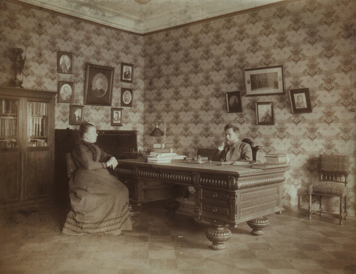
Figure 8. A. A. and Maria Markov in the mathematician’s home office. Family Album 1,
centennial page for A. A. Markov, Jr., August 2003. See more photos in [Basharin et al. 2004].
A Selection of Problems from A.A. Markov’s Calculus of Probabilities: References
Basharin, G. P., A. N. Langville, and V. A. Naumov. 2004, 15 July. The Life and Work of A. A. Markov. Linear Algebra and its Applications 386: 3–26.
Bernstein, S. N. 1927. Sur l'extension du théoréme limite du calcul du probabilités aux sommes de quantités dépendantes. Mathematische Annalen 97: 1–59.
Hayes, Brian. 2013. First Links in the Markov Chain. American Scientist 101(2): 92–97.
Maistrov, L. E. 1974. Probability Theory: A Historical Sketch. Translated by Samuel Kotz. Academic Press.
Markov, A. A. 1900. Calculus of Probabilities (in Russian). St. Petersburg. Subsequent editions: 1908, 1913, and 1924.
Robbins, Herbert. 1955. A Remark on Stirling's Formula. The American Mathematical Monthly 62(1): 26–29.
Seneta, E. 1996. Markov and the Birth of Chain Dependence Theory. International Statistical Review 64(3): 255–263.
A Selection of Problems from A.A. Markov’s Calculus of Probabilities: Acknowledgments and About the Author
Acknowledgments
I would like to thank the librarians at Franklin and Marshall College who found both an online and hard copy of the first edition of this book. With the assistance of a librarian at NYU, they found an online copy of the fourth edition.
I would also like to thank my former student and current colleague, Daniel Droz (F&M ’10, Penn State ’16) for proofreading the translation and typesetting assistance.
About the Author
Alan Levine received his PhD in Applied Mathematics from Stony Brook University in 1983. Since then, he has taught at Franklin and Marshall College, retiring at the end of 2022. He often taught courses in probability and stochastic processes, where Markov's name is featured prominently.
He became interested in translating some of Markov's writings in 2017 when one of his students was completing a joint major in both Russian and mathematics and needed a project to connect the two disciplines. Together, they translated the first three chapters. After the student graduated in 2018—and the subsequent long pause due to COVID—he completed the project in 2022.