An Analysis of the First Proofs of the Heine-Borel Theorem
Introduction
In his 1895 “Sur quelques points de la théorie des fonctions,” Émile Borel (1871-1956) stated for the first time the essential result that has come to be known as the Heine-Borel Theorem in the field of analysis [5, p. 52].
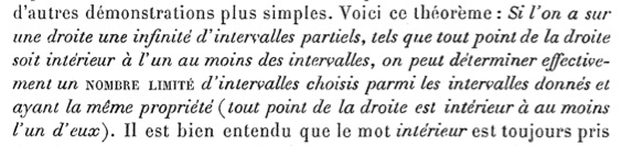
Here is the theorem: If one has on a straight line an infinite number of partial intervals, such that any point on the line is interior to at least one of the intervals, one can effectively determine a LIMITED NUMBER of intervals chosen among the given intervals and having the same property (any point on the line is interior to at least one of them).
Passage 1: The first statement of the Heine-Borel Theorem, along with a translation.
Today we would state this half of the Heine-Borel Theorem as follows.
Heine-Borel Theorem (modern): If a set \(S\) of real numbers is closed and bounded, then the set \(S\) is compact. That is, if a set \(S\) of real numbers is closed and bounded, then every open cover of the set \(S\) has a finite subcover.
 |
 |
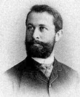
| Eduard Heine (1821–1881), top, and Émile Borel (1871-1956) (Convergence Portrait Gallery) |
Students sometimes struggle with the Heine-Borel Theorem; the authors certainly did the first time it was presented to them. This theorem can be hard to motivate as the result is subtle and the applications are not obvious. Its uses may appear in different sections of the course textbook and even in different classes. Students first seeing the theorem must accept that its value will become apparent in time. Indeed, the importance of the Heine-Borel Theorem cannot be overstated. It appears in every basic analysis course, and in many point-set topology, probability, and set theory courses. Borel himself wanted to call the theorem the “first fundamental theorem of measure-theory” [6, p. 69], a title most would agree is appropriate.
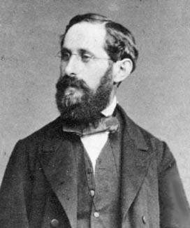
In addition to its mathematical significance, the Heine-Borel Theorem has a complex history. Theophil Hildebrandt (1888-1980) in [11, p. 424] stated, “As in the case of other important mathematical results, the conception of the Borel Theorem is an interesting chapter in mathematical history.” Broadly speaking, the story of the Heine-Borel Theorem has two chapters: pre-1895 and post-1895. In 1989, Pierre Dugac examined letters between the key players and unraveled much of the narrative in his aptly titled “Sur la correspondance de Borel et le théorème de Dirichlet-Heine-Weierstrass-Borel-Schoenflies-Lebesgue” [8]. Of particular interest will be how the theorem got its name given that Eduard Heine (1821–1881) died when Borel was only ten years old.
As with many results, people implicitly used the Heine-Borel Theorem for decades before Borel published it in 1895. David Bressoud noted, “There are two immediate corollaries of the Heine-Borel Theorem that are historically intertwined. They predate Borel’s Theorem of 1895” [6, p. 66]. Bressoud was referring to the Bolzano-Weierstrass Theorem and the theorem that every continuous function on a closed and bounded interval is uniformly continuous (sometimes called Heine’s Theorem), but there were many others as well. Understanding pre-1895 events will help us enrich the classroom experience and empathize with our students’ difficulties. After all, if the importance of the theorem escaped some of the great 19th century analysts, we can forgive our students’ struggles.
In the post-1895 chapter, we see a proliferation of proofs of the Heine-Borel Theorem. Pierre Cousin, William Henry Young, Arthur Schoenflies, and Henri Lebesgue all published proofs within the next nine years. Obviously the later authors and journal editors either were unaware of the earlier publications or were convinced that their arguments improved significantly on what was already in the literature. Up to now, no comparative analysis of the mathematical contributions of these different proofs has been performed. This is the primary goal of our paper.
The story is further complicated because some of the aforementioned five mathematicians published multiple proofs. For example, we know that Borel’s first proof appeared in 1895. From Dugac [8] we know Borel wrote a very similar version in 1898 [3] and two more in 1903 [2] [4]. In our paper, we will concentrate on the first proofs by these authors but will acknowledge subsequent writing when appropriate.
The mathematics of these first proofs is interesting for many reasons. Some have limitations to their usage, whereas others are valid in more general situations. Some are in different dimensions. Some are constructive, and some are purely formal. Some are well written, and others leave out details. We will make particular note of how the different proofs relate to completeness of the real numbers as this connection is indispensable. Recall that the set of real numbers is complete because it has the following equivalent properties [6, p. 62], [1, p. 420]:
- Every sequence of closed, nested intervals has a nonempty intersection.
- Every bounded subset has a least upper bound.
- Every Cauchy sequence converges.
- Every infinite bounded subset has a limit point (Bolzano-Weierstrass property).
- Every monotonic bounded sequence converges (monotone convergence property).
In a modern real analysis course, the second property usually is taken as the definition of completeness, and completeness taken as part of the definition of the real number system. The remaining four properties are then proved as theorems. However, only one of the five mathematicians whose proofs we will discuss used the second property as his definition of completeness. The characterization of completeness that each author assumed is a key difference among the five proofs.
Just as knowing the history can enrich our classroom by shedding light on the difficulties of our students, understanding the mathematics in these proofs can be a valuable teaching tool. So in addition to unraveling the history, our goal is to provide a resource for teachers that will enable them to motivate the study of this essential theorem. This may be achieved in several ways. The teacher may recognize that the proof from her modern textbook is actually from one of these first papers. She can then provide the historical background for what is presented in her text. The instructor may also find that one of these proofs can be more fully integrated into his course than the one he is currently presenting. We hope that he feels free to use these proofs to replace or augment his current presentation. Finally, it makes an excellent project to have students examine a proof that is different from the one presented in their class. Indeed, this paper grew out of just such a project.
An Analysis of the First Proofs of the Heine-Borel Theorem - Introduction
Introduction
In his 1895 “Sur quelques points de la théorie des fonctions,” Émile Borel (1871-1956) stated for the first time the essential result that has come to be known as the Heine-Borel Theorem in the field of analysis [5, p. 52].
Here is the theorem: If one has on a straight line an infinite number of partial intervals, such that any point on the line is interior to at least one of the intervals, one can effectively determine a LIMITED NUMBER of intervals chosen among the given intervals and having the same property (any point on the line is interior to at least one of them).
Passage 1: The first statement of the Heine-Borel Theorem, along with a translation.
Today we would state this half of the Heine-Borel Theorem as follows.
Heine-Borel Theorem (modern): If a set \(S\) of real numbers is closed and bounded, then the set \(S\) is compact. That is, if a set \(S\) of real numbers is closed and bounded, then every open cover of the set \(S\) has a finite subcover.
|
|
|
|
| Eduard Heine (1821–1881), top, and Émile Borel (1871-1956) (Convergence Portrait Gallery) |
Students sometimes struggle with the Heine-Borel Theorem; the authors certainly did the first time it was presented to them. This theorem can be hard to motivate as the result is subtle and the applications are not obvious. Its uses may appear in different sections of the course textbook and even in different classes. Students first seeing the theorem must accept that its value will become apparent in time. Indeed, the importance of the Heine-Borel Theorem cannot be overstated. It appears in every basic analysis course, and in many point-set topology, probability, and set theory courses. Borel himself wanted to call the theorem the “first fundamental theorem of measure-theory” [6, p. 69], a title most would agree is appropriate.
In addition to its mathematical significance, the Heine-Borel Theorem has a complex history. Theophil Hildebrandt (1888-1980) in [11, p. 424] stated, “As in the case of other important mathematical results, the conception of the Borel Theorem is an interesting chapter in mathematical history.” Broadly speaking, the story of the Heine-Borel Theorem has two chapters: pre-1895 and post-1895. In 1989, Pierre Dugac examined letters between the key players and unraveled much of the narrative in his aptly titled “Sur la correspondance de Borel et le théorème de Dirichlet-Heine-Weierstrass-Borel-Schoenflies-Lebesgue” [8]. Of particular interest will be how the theorem got its name given that Eduard Heine (1821–1881) died when Borel was only ten years old.
As with many results, people implicitly used the Heine-Borel Theorem for decades before Borel published it in 1895. David Bressoud noted, “There are two immediate corollaries of the Heine-Borel Theorem that are historically intertwined. They predate Borel’s Theorem of 1895” [6, p. 66]. Bressoud was referring to the Bolzano-Weierstrass Theorem and the theorem that every continuous function on a closed and bounded interval is uniformly continuous (sometimes called Heine’s Theorem), but there were many others as well. Understanding pre-1895 events will help us enrich the classroom experience and empathize with our students’ difficulties. After all, if the importance of the theorem escaped some of the great 19th century analysts, we can forgive our students’ struggles.
In the post-1895 chapter, we see a proliferation of proofs of the Heine-Borel Theorem. Pierre Cousin, William Henry Young, Arthur Schoenflies, and Henri Lebesgue all published proofs within the next nine years. Obviously the later authors and journal editors either were unaware of the earlier publications or were convinced that their arguments improved significantly on what was already in the literature. Up to now, no comparative analysis of the mathematical contributions of these different proofs has been performed. This is the primary goal of our paper.
The story is further complicated because some of the aforementioned five mathematicians published multiple proofs. For example, we know that Borel’s first proof appeared in 1895. From Dugac [8] we know Borel wrote a very similar version in 1898 [3] and two more in 1903 [2] [4]. In our paper, we will concentrate on the first proofs by these authors but will acknowledge subsequent writing when appropriate.
The mathematics of these first proofs is interesting for many reasons. Some have limitations to their usage, whereas others are valid in more general situations. Some are in different dimensions. Some are constructive, and some are purely formal. Some are well written, and others leave out details. We will make particular note of how the different proofs relate to completeness of the real numbers as this connection is indispensable. Recall that the set of real numbers is complete because it has the following equivalent properties [6, p. 62], [1, p. 420]:
- Every sequence of closed, nested intervals has a nonempty intersection.
- Every bounded subset has a least upper bound.
- Every Cauchy sequence converges.
- Every infinite bounded subset has a limit point (Bolzano-Weierstrass property).
- Every monotonic bounded sequence converges (monotone convergence property).
In a modern real analysis course, the second property usually is taken as the definition of completeness, and completeness taken as part of the definition of the real number system. The remaining four properties are then proved as theorems. However, only one of the five mathematicians whose proofs we will discuss used the second property as his definition of completeness. The characterization of completeness that each author assumed is a key difference among the five proofs.
Just as knowing the history can enrich our classroom by shedding light on the difficulties of our students, understanding the mathematics in these proofs can be a valuable teaching tool. So in addition to unraveling the history, our goal is to provide a resource for teachers that will enable them to motivate the study of this essential theorem. This may be achieved in several ways. The teacher may recognize that the proof from her modern textbook is actually from one of these first papers. She can then provide the historical background for what is presented in her text. The instructor may also find that one of these proofs can be more fully integrated into his course than the one he is currently presenting. We hope that he feels free to use these proofs to replace or augment his current presentation. Finally, it makes an excellent project to have students examine a proof that is different from the one presented in their class. Indeed, this paper grew out of just such a project.
An Analysis of the First Proofs of the Heine-Borel Theorem - History
History
As evidenced by the title of Dugac’s canonical paper on the chronology of the Heine-Borel Theorem, “Sur la correspondance de Borel et le théorème de Dirichlet-Heine-Weierstrass-Borel-Schoenflies-Lebesgue,” the list of names associated with the theorem is much longer than just Eduard Heine and Émile Borel. Unfortunately, this paper has not been translated from the French, and so we will review some of its details. Roughly speaking, the contributors can be broken into those who used the theorem (Dirichlet-Heine-Weierstrass) and those who proved the theorem (Borel-Schoenflies-Lebesgue). As we will see, even expanding our scope to consider these six mathematicians will be insufficient.
Certainly the first person to state (and prove) the theorem was Émile Borel (see Passage 1). In the paper “Sur quelques points de la théorie des fonctions” (1895), Borel studied the analytic continuation of functions and came across a “theorem interesting in itself” [10]. Borel deserves extensive credit for stating the result, and his proof is interesting in that it makes use of the transfinite numbers of Georg Cantor (1845-1918). However, the drawback is that he established the theorem only for a countable covering. We will examine his argument carefully in Section 3.
In 1895, the same year that Borel stated and proved his theorem, Pierre Cousin published “Sur les fonctions de n variables complexes” [7]. While stated in a slightly different way from what we see today, elements of the Heine-Borel Theorem were clearly present. In fact, M. R. Sundström stated in [18, p. 7] that, “While Heine is credited with a theorem he did not prove, it appears that Cousin was largely overlooked for a theorem he did prove.”
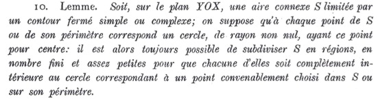
10. Lemma. Define a connected space S bounded by a simple or complex closed contour; if to each point of S there corresponds a circle of finite radius, then the region can be divided into a finite number of subregions such that each subregion is interior to a circle of the given set having its center in the subregion.
Passage 2: Cousin’s version of the Heine-Borel Theorem, along with a translation.
This can be considered a generalization of Borel’s Theorem in two ways. First, Cousin presented the two-dimensional case of the theorem. Also, his proof works for arbitrary coverings. We will translate and analyze his proof in Section 4.
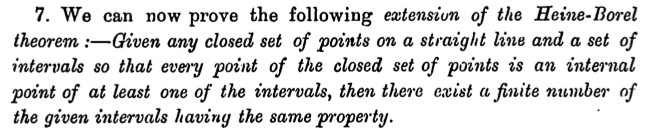
In 1900, Arthur Schoenflies (1853-1928) wrote a report on the development of point-set topology for the German Mathematical Association [15]. He drew attention to Borel’s Theorem, which he said “extends a known theorem of Heine.” This was the first time someone attached Heine’s name to this theorem. It is questionable how similar the “known theorem” actually is to the Heine-Borel Theorem and we will see that this became a source of much contention.
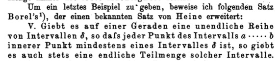
To give a last example, I prove the following theorem of Borel’s, which extends a known theorem of Heine:
V. If on a straight line there is an infinite sequence of intervals \(\delta,\) so that every point of the interval \(a\) ... \(b\) is an interior point of at least one interval \(\delta,\) then there is also always a finite subset of such intervals.
Passage 3: Schoenflies’ version of the Heine-Borel Theorem, along with a translation.
We will examine Schoenflies’ argument in Section 5.
The proof Schoenflies gave followed Borel’s closely, though importantly it did work for arbitrary covers. Hildebrandt wrote, “As a matter of fact, the statement of the Borel Theorem given by Schoenflies in his 1900 Bericht can easily be interpreted to be that of the extension in question” [11, p. 425]. Henri Lebesgue (1875-1941) seemed to agree with Hildebrandt and later advocated to name the theorem Borel-Schoenflies [6, p. 68].
Others disagreed. For example, Paul Montel (1876-1975) wrote, “The name Borel-Schoenflies does not seem to me as justified as that of Heine-Borel: it seems to me that one must distinguish the theorem itself from the applications one might make with it” [8, pp. 105-106]. Borel, for his part, stated in 1903 that, “M. Lebesgue remarked that the hypothesis that the given group is countably infinite is not necessary.” Lebesgue probably said this while teaching a class at Le Collège de France in 1902-1903 [8, p. 99].
In 1902, W. H. Young (1863-1942) published another proof of the uncountable version of the Heine-Borel Theorem [19].
Passage 4: Young’s version of the Heine-Borel Theorem in an article titled “Overlapping intervals.”
Young’s proof depended on a lemma concerning “overlapping intervals.” Once that lemma was proved, the uncountable version of the Heine-Borel Theorem followed immediately. Since this paper is in English and is freely available online, we provide only an analysis in Section 6.
In 1904, Lebesgue gave a wonderfully elegant proof of the theorem in a treatise on integration [14]. Lebesgue had studied Borel’s paper in 1898, but did not notice that the cover needed to be countable. In fact, Lebesgue used the unproved uncountable version in his 1901 thesis. He took the opportunity in 1904 to prove the uncountable version.
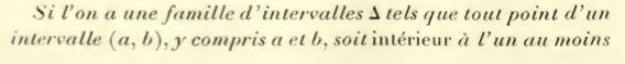
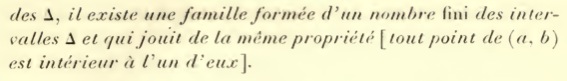
If one has a family of intervals \(\Delta\) such that any point of an interval \(\left(a,b\right),\) including \(a\) and \(b,\) is interior to at least one of \(\Delta,\) there exists a family formed of a finite number of intervals \(\Delta\) and that has the same property [any point of \(\left(a,b\right)\) is interior to one of them].
Passage 5: Lebesgue’s published version of the Heine-Borel Theorem, along with a translation.
A translation of Lebesgue’s modern and simple proof will be found in Section 7. It is this proof that most readers are likely familiar with.
A few years later, Lebesgue reviewed the text The Theory of Sets of Points by W. H. Young (who published the proof of the theorem in Passage 4, above, in 1902) and Grace Chisholm Young [13]. At the end of the review, he turned his attention to “the proposition that the authors, following the example of Messrs. Schoenfliess, Veblen, etc., call the Heine-Borel theorem.” He first explained that he had mistakenly used the uncountable version in 1901.
This demonstration had been obtained in 1898 by M. Vieillefond or by myself, I don’t know anymore, while we were studying together M. Borel’s thesis. I must confess moreover that, although I cited several times M. Borel’s statement, my attention was not held by the word countable that it contains and this is why, in my Thesis, of which the results were published in 1901, I used, without stating it, the modified theorem.
Passage 6a: Lebesgue “confessed” that he missed the word “countable” in Monsieur Borel’s statement.
He then proceeded to attack the attachment of Heine’s name to the theorem. While not the only person to question this association, Lebesgue was probably the most vocal. We’ll review some of the arguments here:
According to Hildebrandt, Schoenflies “noted the relationship of the Borel Theorem to Heine’s proof of the uniform continuity of a function continuous on a closed interval, published in 1872” [11, p. 424]. The name Heine-Borel grew in popularity after it appeared in Young’s proof (Passage 4, above). Lebesgue (Passage 5) did not use Heine’s name. Schoenflies defended his choice in the January 24, 1907 issue of Comptes Rendus, stating that Heine’s uniform continuity theorem is the geometric analogue to Borel’s Theorem [16, p. 22]. Schoenflies sent a copy of this note to Lebesgue prior to publication. Lebesgue wrote back immediately calling the association “ridiculous,” and restated his position in the same journal a few months later [8, p. 105].
Schoenflies’ association of Heine with the theorem was tenuous partly because the connection between Heine and the uniform continuity theorem is itself questionable! Whereas Heine first published the uniform continuity theorem (which does contain a germ of the Heine-Borel Theorem), it was Heine’s professor, Dirichlet, who first realized the uniform continuity theorem and presented the proof in a class he was teaching in 1852. Although Dirichlet’s notes were not published until 1904, Heine wrote a paper in 1872 that gave several results that can be found in those lectures, including the uniform continuity theorem. According to Bressoud, he used “precisely Dirichlet’s argument. Heine did not credit Dirichlet” [6, p. 68].
Lebesgue noted there were many mathematicians in addition to Heine who implicitly used Borel’s Theorem [13, p. 134].
It is therefore not surprising that during arguments made in order to prove such uniformities one incidentally finds demonstrated M. Borel’s theorem; one can cite the reasoning of Heine (Journ. de Crelle, 1872), of M. Goursat (Trans. of the Am. Math. Soc.), of M. Baire (Ann. di Mat., 1900). It is moreover strongly possible that in searching a little, in glancing through, for example, the works of Cauchy, of Seidel, of Stokes, one finds some arguments to cite previous to those of Heine.
Passage 6b: Lebesgue questioned attaching Heine’s name to the theorem.
To the mathematicians Heine, Edouard Goursat (1858-1936), René Baire (1874-1932), Augustin-Louis Cauchy (1789-1857), Philipp von Seidel (1821-96), and George Stokes (1819-1903), we could add the names of Lejeune Dirichlet (1805-59), Karl Weierstrass (1815-97), and Salvatore Pincherle (1853-1936) [6] and probably many others.
Lebesgue disliked crediting people who incidentally used the theorem, noting that the merit was in Borel’s “perceiving it, stating it, and guessing its interest.” He instead offered Borel-Schoenflies. Others campaigned for Borel-Lebesgue, which is still a common name for the theorem. As noted above, Borel himself preferred “the first fundamental theorem of measure theory” [6, pp. 68-69]. It is interesting that Schoenflies eventually caved and dropped Heine’s name from the 1913 edition of his 1900 book [11, p. 424].
Finally, the reader may notice that the word “compact” never appears in these theorems, though it is often found in modern statements of the Heine-Borel Theorem. Fréchet introduced this terminology in 1906 [18, p. 10], and so none of these proofs, published from 1895 to 1904, contained that language.
Let us now turn our attention to the proofs.
An Analysis of the First Proofs of the Heine-Borel Theorem - Borel's Proof
Borel's Proof
The relevant passage from Borel occurs on pages 51-52 of “Sur quelques points de la théorie des fonctions” [5]. Here, he stated that he had found an easy lemma, but that he would prove it nonetheless because it appeared to be interesting.
One can consider this lemma to be nearly evident; nevertheless, because of its importance, I am going to give a demonstration resting on a theory interesting by itself; there exist other simpler demonstrations. Here is the theorem: If one has on a straight line an infinite number of partial intervals, such that any point on the line is interior to at least one of the intervals, one can effectively determine a LIMITED NUMBER of intervals chosen among the given intervals and having the same property (any point on the line is interior to at least one of them).
Notice that Borel mentioned he would go out of his way to provide a proof using a technique that was interesting, rather than using the simplest method. As we work through the proof, we will see that Borel used the monotone convergence characterization of completeness. We should also point out that Borel made a few assumptions that are not explicit. These assumptions will appear in later proofs as well:
- By “straight line,” Borel referred to an interval containing its endpoints - in other words, a closed and bounded interval. Students should be able to find counterexamples if this hypothesis is omitted.
- By “partial intervals,” he meant “open intervals.”
- By “LIMITED NUMBER,” he meant “finite number.”
Borel started by stating his assumption that the cover be countable.
It is as a matter of course that the word interior is always taken in the limited sense which excludes the extremities; it is easy to assure that, without this, the theorem would not be true. One can demonstrate directly that any point on the line is necessarily within the interior of a finite number (supposing the numbered intervals follow an ordinary law [are countable]), but the following demonstration appears to be more in the nature of things.
In the following passage, Borel let the closed, bounded interval be \(\left[A,B\right].\) He let \(\left(A_i,B_i\right)\) be one of the open intervals that contains \(A.\) If \(\left(A_i,B_i\right)\) doesn’t cover \(\left[A,B\right],\) then \(B_i\) is a point in the interior of \(\left[A,B\right]\) or is \(B\) itself. Let \(\left(A_{i_1},B_{i_1}\right)\) be one of the open intervals that contains \({B_i}.\) If \(B_{i_1}\) is less than or equal to \(B,\) then let \(\left(A_{i_2},B_{i_2}\right)\) be one of the intervals containing \(B_{i_1}.\) We continue in this fashion, stopping if we have covered \(\left[A,B\right].\)
Take the left endpoint \(A\) on the line, and let \(\left(A_i,B_i\right)\) be one of the intervals which contains the point \(A\); similarly let \(\left(A_{i_1},B_{i_1}\right)\) be one of the intervals which contains the point \(B_i\), let \(\left(A_{i_2},B_{i_2}\right)\) be one of the intervals which contains the point \(B_{i_1}\) etc. We suppose, as a matter of course, that \(A\) always designates the endpoint left of the intervals, \(B\) the endpoint right.
Notice that the process may terminate at this stage. Namely:
Case 1: If \(B_i\) is greater than \(B,\) or if \(B_{i_n}\) is greater than \(B\) for some \(n,\) then we have a finite cover of \(\left[A,B\right]\) given by \(\left(A_i,B_i\right)\) or by \(\left(A_i,B_i\right),\) \(\left(A_{i_1},B_{i_1}\right),\) \(\left(A_{i_2},B_{i_2}\right),\) ...,\(\left(A_{i_n},B_{i_n}\right),\) respectively. In Diagram 1, this would mean only the purple open set and a finite number of red intervals, including at least one purple or red interval with a right hand endpoint greater than \(B,\) are needed to cover \(\left[A,B\right].\)

Diagram 1: In our diagram of Borel’s argument, we see the closed interval \(\left[A,B\right],\) along with some of the open sets. Left endpoints are listed below the line and right endpoints and limit ordinals are above the line.
Otherwise, Borel examined the sequence of right endpoints \(B_{i_n}.\) This sequence is infinite (else we are in Case 1 above), bounded, and increasing, and thus converges. This is immediate by the monotone convergence property but can also be shown using a bit more work and the Bolzano-Weierstrass property. Borel called the limit \(B_{i_{\omega}}\) (our first limit ordinal, above the green arrow in Diagram 1) and it is the supremum of the set \(\{B_{i_n}\}.\) Because the increasing sequence of right endpoints is bounded above by \(B,\) we know \(B_{i_{\omega}}\) is in \(\left[A,B\right].\) At this point, again the process may terminate:
Case 2: If \(B_{i_{\omega}}\) is equal to \(B,\) then we can form a finite cover in the following way. Obviously \(B\) and therefore \(B_{i_{\omega}}\) is contained in some open interval, which Borel called \(\left(A_{i_{\omega +1}},B_{i_{\omega+1}}\right).\) Since \(B_{i_{\omega}}\) is a limit, only a finite number of the \(B_{i_n}\) lie outside of \(\left(A_{i_{\omega +1}},B_{i_{\omega+1}}\right).\) Borel said that (for example) \(A_{i_{\omega +1}}\) lies between \(B_{i_{m-1}}\) and \(B_{i_m}.\) Therefore, the finite number of intervals \(\left(A_i,B_i\right),\) \(\left(A_{i_1},B_{i_1}\right),\) \(\left(A_{i_2},B_{i_2}\right),\) …, \(\left(A_{i_{\omega}},B_{i_{\omega}}\right),\) \(\left(A_{i_{\omega +1}},B_{i_{\omega+1}}\right)\) cover the subinterval \(\left[A,B_{i_{\omega}}\right].\) In the case when \(B_{i_{\omega}}\) is \(B,\) this shows that a finite number of intervals covers the original interval. In Diagram 1, this would mean we need only one green open interval, one purple, and a finite number of red to cover \(\left[A,B\right].\)
The points \(B_{i_1},\) \(B_{i_2},\) \(B_{i_3},\) …, if they do not reach the extremity \(B\) of the line, have a limit \(B_{i_{\omega}}\) and this point is contained in an interval \(\left(A_{i_{\omega +1}},B_{i_{\omega+1}}\right)\) such that \(A_{i_{\omega +1}}\) falls, for example, between \(B_{i_{m-1}}\) and \(B_{i_m};\) we will be able to disregard the intervals \(\left(A_{i_{m+k}},B_{i_{m+k}}\right),\) and we will have all the same an uninterrupted series of intervals on the line. We will continue similarly, passing to the limit when this is necessary and showing then that one can keep only a finite number of the already considered intervals.
If \(B_{i_{\omega}}\) and \(B_{i_{\omega +1}}\) are less than \(B,\) then we continue in this fashion. Borel already showed there was an infinite sequence of right endpoints \(B_i,\) \(B_{i_1},\) \(B_{i_2},\) … converging to \(B_{i_{\omega}}.\) By repeating the process starting with \(B_{i_{\omega}}\) (instead of \(B_i\)) we get an infinite sequence \(B_{i_{\omega+1}},\) \(B_{i_{\omega+2}},\) ... that converges to \(B_{i_{2\omega}}.\) This process could terminate here as well:
Case 3: If \(B_{i_{2\omega}}\) is equal to \(B,\) we can form a finite subcover of \(\left[A,B\right]\) in the following way. The passage above shows that we can cover \(\left[A,B_{i_{\omega}}\right]\) with a finite number of intervals. The argument in Case 2 then shows that we can cover \(\left[B_{i_{\omega}},B_{i_{2\omega}}\right]\) with a finite number of intervals. These two finite collections of intervals, taken together, cover \(\left[A,B\right].\) In Diagram 1, this means one purple, one blue, and a finite number of red and green intervals are needed to cover \(\left[A,B\right].\)
Assuming \(B_{i_{2\omega}}\) is less than \(B,\) Borel used the above process again, obtaining a sequence \(B_{i_{2\omega+1}},\) \(B_{i_{2\omega+2}},\) ..., converging to a limit \(B_{i_{3\omega}},\) which must be less than \(B\) (otherwise, we can use the technique of Cases 2 and 3 to get a finite cover). After exhausting all the \(B_{i_{m{\omega}+n}},\) he moved on to \(B_{i_{{\omega}^2}},\) ..., \(B_{i_{{{\omega}^2}+n}},\) ..., \(B_{i_{m{{\omega}^2}+n}},\) ..., \(B_{i_{{\omega}^p}},\) ..., \(B_{i_{{\omega}^{\omega}}},\) ..., all of which must be less than \(B\) (else we are done by the above analysis). This brings us to Case 4.
Case 4: Assume that all of the limit points are less than \(B.\) Borel stated that by looking at the right endpoints, he had created a surjection from the open cover to the sequence of right endpoints. Contained within the indices of the right endpoints are the following:
\[B_{i_1}, B_{i_2}, \dots,B_{i_{\omega}}, B_{i_{2\omega}}, \dots,B_{i_{{\omega}^2}}, \dots,B_{i_{{\omega}^{\omega}}}, \dots\]
which consists of all numbers of the second class (ordinals which have no immediate predecessor, or limit ordinals). Because the second class of numbers is not countable, and our original set was, he had arrived at a contradiction [17].
I say that we will necessarily reach the endpoint \(B\) of the line, because, if one did not reach it, one would define a series of intervals having for endpoints \[B_{i_1}, B_{i_2},\dots,B_{i_{\omega}}, B_{i_{2\omega}}, \dots,B_{i_{{\omega}^2}}, \dots,B_{i_{{\omega}^{\omega}}},\] the indices being all the numbers of the second class of numbers (defined by M. Cantor). But these indices are also in a certain order, the natural numbers, in entirety or in part. This is a contradiction because the second class of numbers constitutes a set of the second power.
One must be careful, because in actuality there need not be an interval with right endpoint of \(B_{i_{\omega}},\) \(B_{i_{2\omega}},\) \(B_{i_{{\omega}^2}},\) etc. It is not clear exactly what correspondence Borel referred to in this passage. On one hand, we can create a correspondence between limit ordinals and intervals in the following way
\[{B_{\alpha}}\leftrightarrow\left({A_{\alpha+1}},{B_{\alpha+1}}\right)\]
because these numbers do have successors. Or perhaps Borel used \(B_{i_{\omega}}\) to mean both the infinite sequence and the limit simultaneously. In either case, the flaw isn’t fatal, and he arrived at a contradiction for Case 4, thus completing the proof.
Here is an overview of Borel’s argument, which may be particularly useful to a teacher considering presenting this proof in class.
Background:
- Completeness in the form of the monotone convergence property or perhaps the Bolzano-Weierstrass property is needed to show that the right endpoints have a limit.
- If presenting this proof, some cardinality issues must first be addressed. In particular, definitions of countable, ordinals, ordinal numbers of the second type, etc. will be necessary.
Benefits:
- This is the first statement and proof of the Heine-Borel Theorem and so has the benefit of priority.
- We mentioned that there is a connection between the Heine-Borel Theorem and completeness. As Hallet noted,
It was the original transfinite numbers proof which first established this connection. What the original proof shows, in effect, is that the Bolzano-Weierstrass theorem employed a transfinite (but countable) number of times entails the Heine-Borel property. [9, p. 23]
- Koetsier and van Mill wrote that “Borel’s proof still counts as one of the first applications of transfinite ordinal numbers outside of set theory” [12]. Ironically, while students may feel that the Heine-Borel Theorem is too abstract, it is an application of another abstract area of mathematics, namely Cantorian set theory.
- In his 1898 restatement of his theorem, Borel mentioned that his proof was constructive and that it could be useful in actually creating the finite open cover [3, p. 42].
Passage 7. Borel noted that his proof was constructive.
Lebesgue in [13, p. 133] concurred, stating, “[I]t provides a regular procedure for forming the family, which is only logically defined by the other demonstrations which one gave.” Students who find the Heine-Borel Theorem too abstract may appreciate that this technique gives an explicit covering.
Drawbacks:
- The major drawback of the theorem is that it is not stated, or proved, in its full generality.
- Providing a discussion of Cantor’s ordinal numbers may be a drawback if it is not naturally included elsewhere in the course.
- Borel left out some of the finer points of the proof, which we have tried to remedy here. Having stated that “Borel actually gives very few of the details …” [9, pp. 23-24], Hallet also expanded on the proof.
Impression:
We believe that if the Heine-Borel Theorem is being taught during a set theory or measure theory course, this may be a particularly valuable proof to present. In addition, the constructive nature of the proof may benefit more computationally minded students.
Later Proofs:
Three years later, Borel published Leçons sur la théorie des fonctions [3]. Here he restated the theorem more carefully, noting that the covering must be countable in the statement of the theorem, rather than later in the proof. The proof he presented utilized the nested interval form of completeness and the “divide and conquer” technique that we will see in Cousin’s 1895 proof in the next section.
In May 1903, in “Sur l'approximation des nombres par des nombres rationnels” [4], Borel restated his theorem for arbitrary closed sets, not just intervals. He also mentioned that Lebesgue recognized that the covering need not be countable.
Define, in a space of n dimensions, a countable infinity of closed groups (that is to say such that each one contains its derivative) E1, E2,…,Ep,…, and an ordinary group E such that any point in E is interior to one of Ei. One can, therefore, choose among the Ei a limited number of groups such that any point of E is interior to one of them.
This theorem again, is not quite right – the set E needs to be closed and bounded. Certainly Borel used this fact in his proof, but Ernst Lindelöf (1870-1946) brought it to his attention in a letter on August 24, 1903 [8, p. 99]. When Borel published "Contribution à l’analyse arithmétique du continu" [2] later that year, he included the correct statement of the theorem.
Let E be a given closed and bounded group, E1, E2,…,Ep,…, a countable infinity of groups such that any point of E is interior to, at minimum, one of them; it is possible to find, among E1, E2,…,Ep,…, a limited number of groups such that any point of E is interior to, at minimum, one of them.
An Analysis of the First Proofs of the Heine-Borel Theorem - Cousin's Proof
Cousin's Proof
In his 1895 “Sur les fonctions de n variables complexes,” Pierre Cousin [7] extended the Heine-Borel Theorem to arbitrary covers. On page 22, he wrote:
Define a connected space S bounded by a simple or complex closed contour; if to each point of S there corresponds a circle of finite radius, then the region can be divided into a finite number of subregions such that each subregion is interior to a circle of the given set having its center in the subregion.
Before we examine the proof, we mention a few points:
- According to Dugac, this memoir was completed on October 28, 1893 (two years before Borel), but was not published until 1895 [8, p. 97]. It is very unlikely that Cousin was aware of Borel’s statement and he certainly did not make any reference to it. It appears that Cousin has at least some claim of priority for the theorem.
- Cousin’s statement is a higher-dimensional version of the Heine-Borel Theorem. Circles of finite radius would be equivalent to open intervals in one dimension.
- As Cousin did not work with the real number line in his proof, the form of completeness he used is not precisely one of those listed in our Introduction. However, there are higher-dimensional analogues of these characterizations. Specifically, Cousin made use of the following higher-dimensional version of the nested interval property:
Every nested sequence of closed, bounded sets in \({\mathbb R}^2\) has a non-empty intersection.
- It would be more accurate to refer to his “circles” as “disks” because they do not consist just of the boundary.
- No mention of countability of the cover is made, nor is it required, for this proof.
Cousin started immediately with a description of his proof technique, just as we teach our students to do, and proceeded by contradiction. He used the “divide and conquer” technique that probably appears elsewhere in a real analysis course.
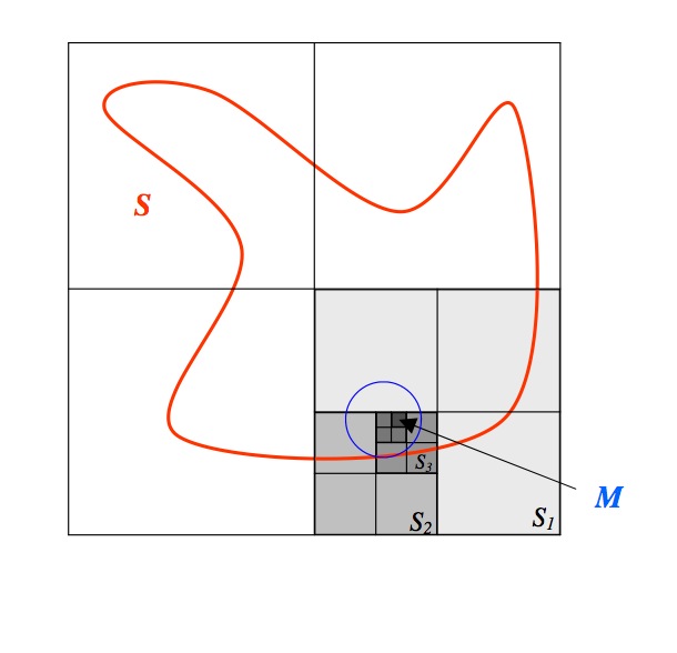
Diagram 2: In this diagram we see the “divide and conquer” method that Cousin employed in his proof.
Cousin took the region S and divided it into \(n>1\) subregions (\(n\) an integer). If the entire region required an infinite number of circles to cover it, then at least one of the subregions must also require an infinite number of circles to cover it. Cousin called that subregion S1. It is the light grey, lower right quadrant of Diagram 2.
We suppose, in fact, the lemma is false: we divide S into squares using parallels to the coordinate axes, in a way that the number of obtained regions is at least equal to a certain integer n; there is at least one of these regions S1, for which the lemma is still false.
Cousin then iterated the process, dividing S1 into n sub-subregions. At least one of these sub-subregions must require an infinite number of circles to cover it. He called this region S2 (the slightly darker grey, lower left quadrant of S1 in Diagram 2.) By continuing in this fashion, he created an infinite sequence of nested closed square regions S1 , S2 , … , Sp , … (the successively darker grey regions in Diagram 2.) He then applied the nested interval property to show there is a point M that is common to each of these Sp, and that M is in the interior or boundary of S.
Subdividing S1 into squares and portions of squares in number at least equal to n, I deduce S2, in the same way that S1 is deduced from S; in following the reasoning, I arrive at an indefinite series of squares or portions of squares S1 , S2 , … , Sp , … ; it is clear that Sp, for p increasing indefinitely, has for a limit a point M interior to S or on its perimeter; ...
Because M is in each Sp, and each Sp cannot be covered by a finite number of circles, certainly each Sp cannot be covered by a single circle. However, as Cousin noted, this is impossible, because M is in S and so some circle of positive radius covers it (the blue circle in Diagram 2). That circle will contain some Sn and all subsequent Sn+k, which is a contradiction to the way that the Sp were constructed.
... one arrives at this conclusion that one can find a square Sp surrounding M or adjacent to M which is not contained in the interior of one of the circles of the statement; however this is impossible because to the point M corresponds a circle of finite radius having this point for a center.
The following may be helpful when considering using Cousin’s proof in a class.
Background:
- A discussion of completeness in the form of the nested interval property applied to nested, closed, bounded, connected two-dimensional regions will be required.
Benefits:
- This proof has the benefit of using the “divide and conquer” technique with which students may be familiar, particularly from Bolzano-Weierstrass or one of the corollaries that we discussed above. If they have not already seen this technique, it is more likely it will appear in their studies than the “numbers of the second type” technique employed by Borel.
- Glancing through introductory analysis, topology, and set theory textbooks shows it is common to see a proof of the Heine-Borel Theorem using a technique similar to the one utilized by Cousin. Presenting Cousin’s proof as the germ of the texbook technique may be helpful for students. Recall that Borel also published a proof using this “divide and conquer” technique in [3]. While appearing years after Cousin’s paper, interested instructors may consider examining Borel’s presentation as well.
- This proof does not require the covering to be countable.
- Even if the course requires only the one-dimensional theorem, it makes for a nice student project to study a higher-dimensional analogue.
- Cousin provided a well-written proof that is easy to follow. His strategy is clearly presented at the beginning and the contradiction is noted at the end.
Drawback:
- Although Cousin’s statement is equivalent to the Heine-Borel Theorem, it certainly is not in the form that students will be using in a basic analysis course. The theorem will need to be translated into the one-dimensional case for most of the applications.
Impressions:
We believe that this proof would be particularly applicable if the Heine-Borel Theorem is being taught in a point-set topology course or in an advanced calculus class where domains of functions are often two-dimensional or higher.
An Analysis of the First Proofs of the Heine-Borel Theorem - Schoenflies' Proof
Schoenflies' Proof
The next proof is due to Arthur Schoenflies in an 1899 review of point-set topology that he wrote for the German Mathematical Association [15]. In practice, this proof is very similar to that of Borel, though it contains more details. Schoenflies assumed the same monotone convergence version of completeness as Borel. Before stating the theorem, he attached both Borel's and Heine’s names to it:
To give a last example, I prove the following theorem of Borel’s, which extends a known theorem of Heine:
V. If on a straight line there is an infinite sequence of intervals \(\delta,\) so that every point of the interval \(a \dots b\) is an interior point of at least one interval \(\delta,\) then there is also always a finite subset of such intervals.
In the following passage, Schoenflies chose an arbitrary point \(a_1\) in the interval and took \(\delta_1\) to be any interval containing it. He looked at the left endpoint \(a_2\) of \(\delta_1\) and let \(\delta_2\) be any interval containing \(a_2.\) Continuing to the left in this fashion, he obtained a sequence of points \(a_1,\) \(a_2,\) … . Assuming that \(a\) is not reached in a finite number of steps (else \(\left[a, a_1\right]\) is covered by a finite number of intervals and we can proceed by looking to the right of \(a_1\)), then the sequence of left endpoints is infinite, decreasing, and bounded below by \(a.\) By either the monotone convergence or Bolzano-Weierstrass properties, it must have a limit point, which he called \(a_{\omega}.\)
Let \(a_1\) be an arbitrary point and \(\delta_1\) an accompanying interval and, further, let \(a_2\) be the left endpoint of \(\delta_1\) and \({\delta}_2\) its accompanying interval. Likewise let \(a_3\) be the left endpoint of \({\delta}_2\) etc. If \(a\) is not yet arrived at by means of a finite number of intervals \(\delta_1,\) \({\delta}_2\)... \({\delta}_{\gamma},\) then the points
\(a_1\), \(a_2\), \(a_3\)…\(a_{\gamma}\)…
have a limit \(a_{\omega}\) which belongs to an interval \({\delta}_{\omega}.\)
Schoenflies continued by applying the same technique to \(a_{\omega}\) and \({\delta}_{\omega},\) and obtained an infinite sequence of points
\(a_1\), \(a_2\), …, \(a_{\omega},\) …, \(a_{\alpha},\) …
which he said was countable by a previous theorem.
Then let \(a_{\omega+1}\) be the left endpoint of \({\delta}_{\omega},\) \({\delta}_{\omega +1}\) the accompanying interval and \(a_{\omega+2}\) its left endpoint etc. We then arrive at a well defined sequence of points ...
\(a_1\), \(a_2\),…\(a_{\omega},\)…\(a_{\alpha},\)…
respectively of intervals...
\(\delta_1,\) \(\delta_2,\)…\({\delta}_{\omega},\)…\({\delta}_{\alpha},\)…
that according to the theorem from p. 13 is countable and hence, necessarily stops at a definite \(\alpha.\)
This meant that the sequence of ordinals he had created must eventually terminate, else he would get an uncountable list of \({\delta}_n,\) which is a contradiction. Notice that this is not the same as saying that the list is finite, just that eventually the list of limit ordinals must end.
The following is the "theorem from p. 13" to which Schoenflies referred.
IV. Each infinite set \(G\) of intervals of a continuous space \(C_v,\) which lie exterior to each other or at most intersect at their borders, is countable.
Schoenflies didn’t give details of the proof, but the result is standard and can be left as an exercise to students. It often proceeds as follows: If one starts with a set of non-overlapping intervals, then each one must contain a rational number. By choosing a rational number \(r_i\) in each \(\delta,\) one can create a one-to-one correspondence between the intervals and a subset of the rational numbers. Because the rational numbers are countable, so is the subset, and hence so is the set of non-overlapping intervals.
In this case, it is not clear why this theorem is relevant. After all, the intervals \({\delta}_n\) can overlap! Schoenflies actually applied this theorem to the intervals \(\left(a_i, a_{i+1}\right)\) writing, “Namely if \(a_1\) > \(a_2\) > \(a_3\) . . . . is a sequence of positive numbers decreasing to zero without end, then the intervals whose content is between \(a_{\nu}\) and \(a_{\nu +1}\) …” [15, p. 13]. Because these intervals don’t overlap, they are countable and so are the \(a_i.\) In Young’s proof in the next section we will see another trick that would have allowed Schoenflies to apply this theorem directly.
Let us return to the main theorem. After claiming that the sequence of \({\delta}_n\) is countable, Schoenflies argued that he could replace this infinite list of intervals with a finite list. He started by showing that he could cover \(\left[a_{\omega}, a_1\right]\) by a finite number of intervals. Because \(a_{\omega}\) is a limit point, then an infinite number of the \(a_i\) lie within \({\delta}_{\omega}.\) In other words, there exists a number \(\mu\) so that all \(a_i\) with \(i\ge\mu\) will lie within \({\delta}_{\omega}.\) Therefore \(\left[a_{\omega}, a_1\right]\) will be covered by the finite set of intervals \({\delta}_1,\) \({\delta}_2,\) …, \({\delta}_{\mu},\) \({\delta}_{\omega}.\)
Now this sequence of intervals can always be substituted by a finite set of analogous intervals. Returning first to point \(a_{\omega},\) there is certainly a number \(\mu\) so that all points \(a_{\nu}, a_{\nu +1},\) ... lie within \({\delta}_{\omega}\) and hence, the interval \(a_1\) ... \(a_{\omega}\) is covered already by the intervals \({\delta}_1,\) \({\delta}_2,\)…\({\delta}_{\mu},\) \({\delta}_{\omega}.\)
He argued that this process of reduction to a finite number of intervals does not work just when passing from the finite numbers to \(\omega,\) but whenever \(a_{\beta}\) is a limit ordinal - that is, a limit of a strictly decreasing sequence of left endpoints. The details of the induction are missing. Hallet filled in the holes, noting that, “he only proves the induction step from finite numbers to \(\omega,\) and not in complete generality” [9, p. 22].
However, this is true for every point \(a_{\beta}\) which is the limiting point of a sequence \[a_{\alpha_1}, a_{\alpha_2}, a_{\alpha_3}, \dots, a_{\alpha_v},\dots\] so that the terminus of \(\{a_{\alpha_v}\}\) satisfies that \(a_{\alpha_{\omega}} = a_{\beta}.\) Assuming namely that every \(a_{\alpha_{i+1}}\) from \(a_{\alpha_i}\) on can be arrived at via a finite number of intervals, then this is also true of \(a_{\beta}\) because again \(a_{\beta}\) belongs to an interval \({\delta}_{\beta},\) and there is a definite \(\mu\) with all points \(a_{\alpha_{\mu}},\) \(a_{\alpha_{\mu+1}},\dots\) belonging to \(a_{\beta}.\) Now since the intervals \(\delta\) should also contain the endpoints \(a\) and \(b,\) the claim is proved.
It is clear that this proof is very similar to Borel’s, though it does make a rather clumsy argument that the original cover need not be countable. Immediately upon completing the proof, Schoenflies stated that the theorem is also true in higher dimensions, and proceeded to sketch how the proof would proceed. It is different from the two dimensional argument of Cousin, for Schoenflies required the use of the one-dimensional theorem. Some of the details are missing, but it can make for a good project for students to unravel the proof.
It is not difficult to apply the same theorem to planes and spaces. Namely, if \(a_1\) is now a point of a rectangle \(H\) and \({\delta}_1\) the region around it, which for the sake of simplicity I shall consider as a square, then to every point \(a_2\) on he perimeter of \({\delta}_1\) there also belongs such a square \({\delta}^{\prime}_1\) and it follows from the proven theorem, that there exists a finite number of squares such that all points \(a_2\) on the perimeter of \({\delta}_1\) become interior points of one of these squares. There exists therefore in any case also a square \({\delta}_2\) which encloses \({\delta}_2\) such that all points within and on the perimeter of \({\delta}_2\) are covered by a finite number of squares. For this square there exists an analogous square \({\delta}_3\) etc. and the proof proceeds analogously to the proof above. Here as well every point of the perimeter of \(H\) must belong to a region \({\delta}.\)
As before, we now provide details of the argument that teachers may consider before presenting this argument in a classroom.
Background:
- If teaching this proof, one must cover completeness in the sense of the monotone convergence property or the Bolzano-Weierstrass property to show that the left endpoints have a limit.
Benefits:
- This proof closely follows that of Borel, though it does not require that the original cover be countable.
- Similarly to Borel’s proof, it offers a nice application of Cantor’s ordinal numbers.
- The outline of the generalization to two dimensions (or even more) would make a valuable project for students to work though.
Drawbacks:
- The step where Schoenflies proved that the covering must be countable is buried in a different section. And, it is not immediately clear how to apply that theorem. Details certainly need to be provided for a student to understand the full proof.
- As Hallet wrote, Schoenflies omitted several details in the induction step that an instructor would need to fill in.
Impressions:
As in the case of Borel’s original proof, this proof may be particularly relevant if the theorem is covered in a set theory or measure theory course.
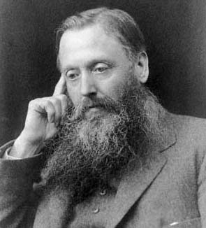
Arthur Schoenflies (1853-1928) (Convergence Portrait Gallery)
Later Proofs:
A few years later in 1907, Schoenflies published another note, “Sur un théorème de Heine et un théorème de Borel” [16]. As we mentioned above, it was in this paper that he took the opportunity to defend his choice of attaching Heine’s name to the theorem. He also gave another proof, which is interesting as well. Around every point p of a closed set P, he defined ρ to be the greatest radius of an interval containing p. He then showed that the lower limit of all the ρ was not zero. He proceeded, saying “In fact, if this limit were zero, one could choose points p1, p2, …, pγ, in such a manner that the radii ρ1 > ρ2 > … > ργ … converge to zero. Let \(p_{\omega}\) be a limit point of { pγ }; for this point there exists a radius \({\rho}_{\omega}>0\) and forcing the well-known contradiction.”
Schoenflies didn’t elaborate on the “well-known” contradiction, but it may proceed along these lines: let U be the open interval around \(p_{\omega}.\) It has radius \({\rho}_{\omega}>0.\) Since \(p_{\omega}\) is a limit point there are an infinite number of the points p1, p2, …, pγ in U. Those points form a subsequence of the original sequence, and so would have corresponding radii ρi converging to zero. However, because each point is in the interval around \(p_{\omega},\) each ρi must be at least \({\rho}_{\omega},\) which is fixed so the radii ρi can’t converge to zero.
Once he knew that every point p is contained in an interval with positive radius > δ, Schoenflies could show a finite number would cover. This makes for a nice exercise for students. He also commented that, “This demonstration is exactly the same, whether the supposed set of domains is countable or not” [16, p. 23].
An Analysis of the First Proofs of the Heine-Borel Theorem - Young's Proof
Young's Proof
In 1902, W. H. Young published the paper “Overlapping Intervals” in the Bulletin of the London Mathematical Society [19]. This paper is in English and can be found here (pdf download), so we do not provide a translation. The main point of this paper is the following:
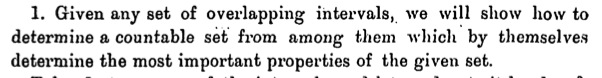
Young did not say exactly what “the most important properties” are, but we can take it to mean the union of the countable intervals is equivalent to the union of the original set of intervals. Notice that nothing is mentioned about the overlapping intervals covering a closed and bounded interval.
Clearly once this theorem has been proved, the uncountable version of the Heine-Borel Theorem follows readily. If one has an uncountable cover of a closed and bounded interval, one can determine a countable cover using Young’s theorem and then apply Borel’s countable version of the Heine-Borel Theorem to complete the proof.
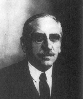
William Henry Young (1863-1942) (Convergence Portrait Gallery)
The proof of Young’s result proceeds very much like Borel’s original proof and assumes the same form of completeness. He started by choosing an arbitrary interval \(d.\) He then chose an interval that “abuts or overlaps with \(d\) on the left” and called it \(d^{\prime}.\) He continued in this fashion moving to the left, constructing \(d^{\prime\prime}, d^{\prime\prime\prime},\) etc. He observed (like Borel and Schoenflies) that the left endpoints of these intervals must have “a limiting point \(P\) external to all of them.” He called this limit point \(D.\) “There will only be a finite number of the intervals \(d, d^{\prime}, d^{\prime\prime},\) which do not overlap with \(D.\) Let \(d^{\left(i\right)}\) be the first which overlaps with \(D,\) then we select the intervals \(d, d^{\prime}, d^{\prime\prime}, \dots, d^{\left(i\right)}, D\) and omit from consideration all the intervals \(d^{i+1}, d^{i+2}, \dots.\)”
He continued this operation with the left endpoint of \(D,\) as well as with the right endpoint of the original starting interval \(d.\) Obviously, in order to prove his main theorem, he wanted to show the resulting cover was countable. In order to do this, he passed from his set of overlapping intervals to a new set of non-overlapping intervals in the following way. Starting with \(d\) and \(d^{\prime}\) he defined \(\delta^{\prime}\) to be \(d^{\prime}\setminus d.\) Similarly, he defined \(\delta^{\prime\prime}\) to be \(d^{\prime\prime}\setminus d^{\prime}.\) Each of these \(\delta\) are non-overlapping, and by “the theory of sets of non-overlapping intervals, can be arranged in countable order.”
Then, because the non-overlapping intervals \(\dots,{{\delta}^{\prime\prime\prime}},{{\delta}^{\prime\prime}},{{\delta}^{\prime}},\dots\) are in one-to-one correspondence with the intervals \(\dots,{d^{\prime\prime\prime}},{d^{\prime\prime}},{d^{\prime}},\dots,\) he had created a countable (almost) covering. When two successively chosen intervals in the construction abut (don’t overlap), then the point between them will be not be covered by the union of the intervals. Therefore, there are at most a countable number of points \(p_1,p_2,\dots\) not covered by the intervals determined above. However, each of these \(p_i\) are covered by some interval, so if we append those intervals to the above collection we end up with a countable collection that covers the original union.
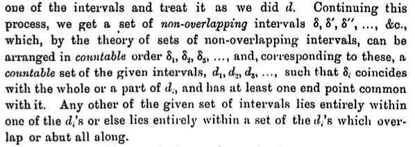
Young did not give any detail about the “theory of sets of non-overlapping intervals” but we assume the theorem is exactly the one that Schoenflies referred to in his Bericht.
As above, here are the relevant details of Young’s proof:
Background:
- A discussion of completeness in the form of the monotone convergence property or the Bolzano-Weierstrass property is necessary to understand the proof.
- Some presentation of the “theory of non-overlapping intervals” needs to be done. This step could probably be an exercise to the students, as long as they know some very basic cardinality.
Benefits:
- Young does not require the covering to be countable.
- The proof starts like Borel’s and Schoenflies’ proofs, but the key step requires much less background.
- As with the other similar proofs, Young’s technique is constructive.
- It is in English and is easy to follow.
Drawback:
- This proof is not self-contained. Although the proof does reduce an arbitrary cover to a countable cover, one must then apply Borel’s proof to this countable cover. For a complete argument, both Young and Borel must be taught.
This proof features many of the benefits of the Borel and Schoenflies proofs, but without the drawback of needing advanced set theory. If Borel’s proof has already been covered, this is a quick argument showing the cover need not be countable.
An Analysis of the First Proofs of the Heine-Borel Theorem - Lebesgue's Proof
Lebesgue's Proof
In 1904, Lebesgue published his version of the theorem [14], which he said was due to Borel.
To compare the two numbers me, mi, we will use a theorem attributed to M. Borel:
If one has a family of intervals Δ such that any point on an interval (a,b), including a and b, is interior to at least one of Δ, there exists a family formed of a finite number of intervals Δ and that has the same property [any point of (a,b) is interior to one of them].
Note that where Lebesgue wrote (a,b) for a closed and bounded interval, we would write [a,b]. Unlike his predecessors, Lebesgue assumed the least upper bound property as his characterization of completeness.
In the passage shown below, Lebesgue started by presenting a new definition - that if [a,x] can be covered by a finite number of subintervals, then x is reached. In his notation, if x is reached, then so are all points between a and x. If x is not reached, then neither are any of the points between x and b (because if there were a y between x and b that was reached, then [a,y] would be covered by a finite number of subintervals, and so would [a,x]).
Let (á,β) be one of the intervals Δ containing a, the property to demonstrate is evident for the interval (a,x), if x is contained between á and β; I want to say that this interval may be covered with the help of a finite number of intervals Δ, which I express in saying that the point x is reached. It must be demonstrated that b is reached. If x is reached, all the points of (a,x) are [reached]; if x is not reached, none of the points of (x,b) are [reached].
He assumed that b is not reached (else the proof is done), then defined x0 to be the “first point not reached” or the “last point reached”. In modern notation, he defined x0 to be the greatest lower bound of the set \[X=\{x\in\left[a,b\right]\,\vert\,x\,\,{\rm is}\,\,{\rm not}\,\,{\rm reached}\}.\] This set is nonempty and bounded, and therefore has a greatest lower bound .
Now x0 is contained in some interval, which he called (á1,β1). In the following passage, he then chose two points x1 and x2 satisfying α1 < x1 < x0 < x2 < β1. By the definition of x0 he saw that x1 is reached and x2 is not reached. Because x1 is reached, [a, x1] is covered by a finite number of intervals. If we take that collection and append the interval (á1,β1) we get a finite collection that covers x2. This is a contradiction. Therefore b must have been reached.
Let x1 be a point of (á1,x0), x2 a point of (x0,β1); x1 is reached by assumption, the intervals Δ in finite number which are used to reach it, plus the interval (á1, β1) allows x2 > x0; x0 is neither the last point reached, nor the last not reached; therefore b is reached (1).
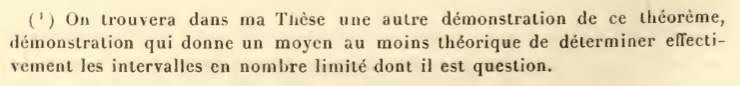
In his footnote, Lebesgue explained Borel’s contributions. He mentioned that Borel required that the covering be countable, and noted that this may sometimes be adequate. However, he felt that the general theorem would be more useful.
(1) M. Borel gave, in his Thesis and in his Lessons on the theory of functions, two demonstrations of this theorem. These demonstrations essentially suppose that the set of intervals Δ are countable; this suffices in some applications; there is however interest in demonstrating the theorem of the text. For example, for the applications that I made in my Thesis of M. Borel’s theorem, it was necessary that he demonstrated for a set of intervals Δ having the power of the continuum.
Finally we give our overview of Lebesgue’s proof.
Background:
- Completeness in the form of existence of the supremum for every non-empty bounded set will be required to carry out this proof.
Benefits:
- This proof is very short and is particularly easy to follow. In fact, starting the proof may lead to an “ah-ha!” moment where the students can complete the necessary steps.
- It appears that those textbooks that don’t use the “divide and conquer” technique of Cousin do use Lebesgue’s method. This proof may integrate particularly nicely into those courses.
- This technique of proof is very useful, and appears, for example, in the intermediate value theorem. If students have not already seen it, it is likely that they will.
- This proof works just as well for countable as uncountable covers.
Drawback:
- The proof is non-constructive. There is no way that we can ascertain the finite covering by working the proof.
Impressions:
This is the one! The proof is thoroughly modern and simple to follow. In comparison, all previous arguments are cumbersome and overly complicated. It is no wonder that many people choose to attach Lebesgue’s name to Borel’s when referencing the theorem. Certainly this proof should be presented in any real analysis course, and probably in many others!
Henri Lebesgue (1875-1941) (Convergence Portrait Gallery)
An Analysis of the First Proofs of the Heine-Borel Theorem - Conclusion
Conclusion
The use of primary sources or historical documents can be a powerful teaching tool in any course. It can provide context and improve retention of the material.
The Heine-Borel Theorem will be familiar to any math major, though many may struggle with the abstractness of the proof. By presenting the historical development along with the mathematics, we may help students understand the theorem. Students often are surprised to learn that this theorem escaped many brilliant mathematicians for decades. They also may enjoy the debate surrounding the name.
Of course, our goal is not merely to provide historical anecdotes. By translating and analyzing historical proofs, we provide teachers with tools to enrich their presentation of this topic in a variety of ways. A teacher may either augment or replace a proof from the textbook. Or projects for students can be developed. Regardless, we believe this information can improve the teaching of this topic.
We hope that readers find this a valuable resource in their classes.
Acknowledgments
The authors would like to thank Dr. Tim Bennett for his help with their translations. They would also like to thank the referees and especially the editor of Convergence for their many helpful suggestions, as well as their patience, in improving this paper.
About the Authors
Nicole Andre is currently a medical student at Ohio University Heritage College of Osteopathic Medicine. She earned her B.S. in Biology at Wittenberg University in Springfield, Ohio, in May of 2012. Along with studying biology she focused on achieving proficiency in the German language and studied for a semester in Marburg, Germany. Upon completing her medical education, Nicole hopes to work as a physician in an underserved area.
Susannah Engdahl is a senior at Wittenberg University, where she is pursuing a major in physics and minors in mathematics and computational science. After leaving Wittenberg, she plans to attend graduate school to study biomedical engineering.
Adam Parker is associate professor of mathematics at Wittenberg University. He has undergraduate degrees in mathematics and psychology from the University of Michigan, and earned his mathematics Ph.D. in 2005 from the University of Texas at Austin under the direction of Dr. Sean Keel. His research interests include algebraic geometry and the history of mathematics.
An Analysis of the First Proofs of the Heine-Borel Theorem - Works Cited
Works Cited
1. Bloch, E. (2011). The real numbers and real analysis. New York: Springer.
2. Borel, É. (1903). Contribution à l’analyse arithmétique du continu. Journal de mathématiques pures et appliquées 5e série, 329-375.
3. Borel, É. (1898). Leçons sur la théorie des fonctions. Paris: Gauthier-Villars.
http://www.archive.org/details/leconstheoriefon00borerich
4. Borel, É. (1903). Sur l'approximation des nombres par des nombres rationnels. Comptes Rendus de l'Académie des Sciences de Paris, 1054-1055.
5. Borel, É. (1895). Sur quelques points de la théorie des fonctions. Annales scientifiques de l'E.N.S. Serie 3, 12, 9-55.
http://www.numdam.org/item?id-ASENS_1895_3_12__9_0
6. Bressoud, D. M. (2008). A radical approach to Lebesgue's theory of integration. New York: Cambridge University Press.
7. Cousin, P. (1895). Sur les fonctions de n variables complexes. Acta Mathematica, 19, 22.
http://dx.doi.org/10.1007/BF02402869
8. Dugac, P. (1989). Sur la correspondance de Borel et le théorème de Dirichlet-Heine-Weierestrass-Borel-Schoenflies-Lebesgue. Archives internationales d'histoire des sciences, 39 (122), 69-110.
9. Hallett, M. (1979). Towards a theory of mathematical research programmes (I). The British Journal for the Philosophy of Science, 30 (1), 1-25.
10. Hawkins, T. (1980). The origins of modern theories of integration. In I. Grattan-Guinness, From the calculus to set theory 1630-1910, an introductory history (p. 175). Princeton: Princeton University Press.
11. Hildebrandt, T. (1926). The Borel theorem and its generalizations. Bulletin of the American Mathematical Society, 423-425.
http://projecteuclid.org/DPubS?service=UI&version=1.0&verb=Display&handle=euclid.bams/1183487130
12. Koetsier, T. and J. van Mill (1999). By their fruits ye shall know them: some remarks on the interaction of general topology with other areas of mathematics. In History of Topology (pp. 199-239). Amsterdam: North-Holland Publishing Company.
13. Lebesgue, H. (1907). Comptes rendus et analyses: Review of Young and Young, The theory of sets of points. Bulletin des sciences mathématiques (2), 31, 132-134.
14. Lebesgue, H. (1904). Leçons sur l'intégration et la recherche des fonctions primitives. Paris.
http://ia600201.us.archive.org/23/items/leconegrarecher00leberich/leconegrarecher00leberich.pdf
15. Schoenflies, A. (1900). Die Entwickelung der Lehre von den Punktmannigfaltigkeiten. In Jahresbericht der deutschen Mathematiker-Vereinigung. Leipzig: B.G. Teubner. Also available from Google Books.
16. Schoenflies, A. (1907). Sur un théorème de Heine et un théorème de Borel. Comptes Rendus de l'Académie des Sciences de Paris, 144, 22-23.
http://gallica.bnf.fr/ark:/12148/bpt6k3098j/f22.tableDesMatieres
17. Stoll, R. R. (1979). Set Theory and Logic. New York, New York, USA: Dover.
18. Sundström, M. R. (2010 21-June). A pedagogical history of compactness.
From arxiv: http://arxiv.org/abs/1006.4131
19. Young, W. H. (1902). Overlapping intervals. Bulletin of the London Mathematical Society, 35, 384-388.
http://plms.oxfordjournals.org/content/s1-35/1/384.full.pdf