When Nine Points Are Worth But Eight: Euler's Resolution of Cramer's Paradox
Overview
Gabriel Cramer and Leonhard Euler both wrote important books on the theory of equations in the mid 18th century. During the years leading up to their publications, they carried on a friendly and fruitful correspondence. One topic they discussed was a paradox that was first noticed by Maclaurin: that nine points should be sufficient to determine a curve of order three, and yet two different curves of order three could intersect in up to nine different places. Although this situation has come to be known as Cramer's Paradox, it was Euler who first suggested the resolution of this apparent contradiction, in a letter that was lost long ago but rediscovered in the Smithsonian Institution in 2003.
In this paper, we investigate the properties of algebraic curves of order two and higher and describe Cramer's Paradox and Euler's resolution, including his elegant example of an infinite family of cubic curves that all pass through the same nine points. We also provide the first English translation of Euler's long lost letter of October 20, 1744.
When Nine Points Are Worth But Eight: Euler’s Resolution of Cramer’s Paradox - Introduction
Two points determine a straight line. There are few mathematical statements so clear and indisputable. Yet even this simple statement needs a little qualification. Although we would generally imagine the two points in question to be different from one another, we should probably make that explicit:
Postulate 1. Two distinct points in the plane determine a unique straight line.
This is similar to the first postulate in Euclid's Elements: "to draw a straight line from any point to any point." His use of the linguistic construction "from … to" suggests that he also meant the two points to be distinct, but he didn't postulate the uniqueness of this line, even though he implicitly used uniqueness, for example in his proof of Proposition XI.3.
In analytic geometry, where we think in terms of algebraic equations instead of geometric constructions, we know how to calculate the equation of a straight line given two distinct pairs \((x_1,y_1)\) and \((x_2,y_2).\) If our concern is to find a linear function \(y=mx+b,\) then Postulate 1 needs the additional qualification that the two points have distinct \(x\)-coordinates.
How does this simple principle generalize to curved lines and larger numbers of points? This vague question can be answered in a number of ways: for example, three points can determine a circle or a parabola. More generally, five points usually determine a conic section; that is, either an ellipse, a parabola, or a hyperbola. Like the corresponding proposition for straight lines, this principle needs some qualification in order that the conic be uniquely determined. And like that result, it can be treated either as a problem in geometry or as a problem in algebra, involving second degree equations in two variables. Of course, this second approach only became possible in the 17th century, after the introduction of analytic geometry.
By the 18th century, mathematicians knew how to generalize this proposition about conic sections to curves of higher order. (We will define equations of degree two and higher later in this paper.) Colin Maclaurin (1698-1746), Gabriel Cramer (1704-1752), and Leonhard Euler (1707-1783) all independently discovered that \(\frac{n^2+3n}{2}\) points determine a curve of order \(n,\) subject to certain conditions. When \(n>2\) there are no geometric constructions; instead, Maclaurin, Cramer, and Euler used a counting argument that comes from considering the equations of such curves. Quite likely, other mathematicians of the time came to the same conclusion by themselves, but at least one of them – William Braikenridge (ca. 1700-1762) – thought that the correct number was actually \(n^2+1.\) We notice that this agrees with \(\frac{n^2+3n}{2}\) only in the two classical cases \(n=1\) and \(n=2.\) Instead of counting coefficients in an equation, Braikenridge's argument came from considering the way in which two lines or curves in the plane can intersect.
When Nine Points Are Worth But Eight: Euler’s Resolution of Cramer’s Paradox - Intersection of Lines and Curves
Two straight lines in the plane intersect in one point. This statement is always true, except when the two lines are parallel (although the statement is always true in the projective plane). And like the previous question, the problem of intersection can be considered for curves of higher degree. For example, a line can typically intersect an ellipse, parabola or hyperbola in two points. Two conics can intersect in as many as 4 points. By considering various low order cases, many 18th century mathematicians came to the conclusion that two curves of order \(m\) and \(n\) typically intersect in \(mn\) points, and can never intersect in more than \(mn\) points. This result is now called Bézout's Theorem, after Etienne Bézout (1730-1783), who gave the first acceptable proof of this result in 1779.
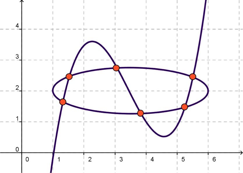
Figure 1. A polynomial of degree three and an ellipse may intersect in six points. (Image created using GeoGebra.)
Hold on, now … there's a problem here! Let's suppose \(m=n=3.\) Then on the one hand, two curves of order three will typically intersect in 9 points. On the other hand, if \(n=3,\) then \(\frac{n^2+3n}{2}=9,\) so those same 9 points should have been enough to determine a unique curve of order three! This apparent contradiction goes by the name of Cramer's Paradox, although it was first noticed by Maclaurin and it was resolved at least as successfully by Euler as it was by Cramer.
In this article, we will look at the problem of fitting points to curves and use some modern notions from linear algebra to understand how Cramer's Paradox is resolved. We will also look at the work of Euler and Cramer, who grappled with this problem but didn't have the benefit of such notions as linear independence and rank in order to guide their thoughts. We will also get a glimpse of a letter that Euler wrote to Cramer in 1744, which had been unknown until 2003 but will soon appear in Euler's collected works, in which Euler first suggested a resolution for Cramer's Paradox.
When Nine Points Are Worth But Eight: Euler’s Resolution of Cramer’s Paradox - Special Case: the Circle
In Book IV of his Elements, Euclid gave one way to generalize the result that two distinct points determine a line. Proposition 5 of that book gives the construction of the circle that circumscribes any given triangle. Because a triangle is determined by three noncollinear points, Euclid's proof essentially says:
Theorem 1. Three noncollinear points in the plane determine a unique circle.
Euclid's proof is entirely geometric. Given a triangle \(ABC,\) he constructed perpendicular bisectors on two of the sides. The point \(F\) where these two lines intersect is called the circumcenter of \(ABC\) and does not depend on which two sides are chosen. Euclid then showed that the distance from \(F\) to each of the points \(A, B\) and \(C\) is the same, say \(r.\) Therefore, the circle with center \(F\) and radius \(r\) passes through all three points \(A, B\) and \(C.\)
Figure 2. A triangle \(ABC,\) together with its circumcircle \(ABC\) and circumcenter \(F.\) Move points \(A, B\) and \(C\) to explore relationships among triangle, circumcircle, and circumcenter. (Interactive applet created using GeoGebra.)
It's interesting to observe that in the case of an obtuse angled triangle, the circumcenter falls outside of the triangle \(ABC.\) Furthermore, if \(ABC\) is a right triangle, then the circumcenter is the midpoint of the hypotenuse, so that the hypotenuse is the diameter of the circle passing through the three points. All of these features can be explored by moving any of the points \(A, B\) or \(C\) in the applet in Figure 2.
After the invention of analytic geometry, it became possible to solve this problem algebraically. A circle with center \((h,k)\) and radius \(r\) satisfies the equation \[(x-h)^2 + (y-k)^2 = r^2,\] so given three noncollinear points with coordinates \((x_1,y_1),\) \((x_2,y_2)\) and \((x_3,y_3),\) we substitute these pairs of numbers to get three equations in the three unknowns \(h,\) \(k\) and \(r.\) Although these equations aren't linear, it's possible to do a little algebra to eliminate the \(r^2\) and get two linear equations in the unknowns \(h\) and \(k,\) which will always have a solution, as long as the given points are not collinear. Rather than work through these details, we'll consider the example of curve fitting with three points and a parabola.
When Nine Points Are Worth But Eight: Euler’s Resolution of Cramer’s Paradox - Special Case: the Parabola
Given three distinct points \((x_1, y_1), (x_2, y_2),\) and \((x_3, y_3),\) we wish to determine the conditions under which there exists a parabola that passes through these points. Specifically, let's consider the case in which the parabola gives \(y\) as a function of \(x.\) In other words, we want to find real numbers \(a, b, c\) such that the equation of the parabola \(y = f(x) = ax^2 + bx + c\) satisfies \(y_i = f(x_i)\) for \(i = 1, 2, 3.\)
First, we observe that for the function \(f\) to exist, the values \(x_i\) must all be distinct, for otherwise we would be assigning two distinct codomain values to a single domain value of \(f.\)
The real numbers \(a, b, c\) exist exactly when there is a solution to the system of equations
\[\begin{eqnarray*}a(x_{1})^{2} + bx_{1} + c & = & y_1 \\a(x_{2})^{2} + bx_{2} + c & = & y_2 \\a(x_{3})^{2} + bx_{3} + c & = & y_3\end{eqnarray*}\]
Because this system of equations is linear in \(a, b, c,\) we may rewrite it as the matrix equation \[\begin{bmatrix}x_1^2 & x_1 & 1 \\x_2^2 & x_2 & 1 \\x_3^2 & x_3 & 1\end{bmatrix}\,\begin{bmatrix}a \\b \\c \end{bmatrix}=\begin{bmatrix}y_1 \\y_2 \\y_3\end{bmatrix},\]
which may be represented by the augmented matrix \[\begin{bmatrix}x_1^2 & x_1 & 1 & y_1 \\x_2^2 & x_2 & 1 & y_2 \\x_3^2 & x_3 & 1 & y_3\end{bmatrix}.\]
We now perform some elementary row operations – subtract the first row from the second row and from the third row: \[\begin{bmatrix}x_1^2 & x_1 & 1 & y_1 \\x_2^2 - x_1^2 & x_2 - x_1 & 0 & y_2 - y_1 \\x_3^2 - x_1^2 & x_3 - x_1 & 0 & y_3 - y_1 \\\end{bmatrix}\]
Because we know that \(x_1\neq x_2\) and \(x_1 \neq x_3,\) we may divide the second and third rows by \(x_2 - x_1\) and \(x_3 - x_1,\) respectively. This gives\[\begin{bmatrix}x_1^2 & x_1 & 1 & y_1 \\x_2 + x_1 & 1 & 0 & {\displaystyle \frac{y_2 - y_1}{x_2 - x_1}} \\x_3 + x_1 & 1 & 0 & {\displaystyle \frac{y_3 - y_1}{x_3 - x_1}} \\\end{bmatrix}\]
Finally, we subtract the second row from the third row, and obtain:\[\begin{bmatrix}x_1^2 & x_1 & 1 & y_1 \\x_2 + x_1 & 1 & 0 & {\displaystyle \frac{y_2 - y_1}{x_2 - x_1}} \\x_3 - x_2 & 0 & 0 &{\displaystyle \frac{y_3 - y_1}{x_3 - x_1} - \frac{y_2 - y_1}{x_2 - x_1}} \\\end{bmatrix}\]
Because \(x_2\neq x_3,\) we see that the system of equations represented by this augmented matrix is consistent, and moreover, that the solution for \(a, b, c\) is unique. Therefore, there is a unique curve with equation \(y = ax^2 + bx + c\) that passes through the given points.
But is this curve really a parabola? Only if \(a\ne 0\); otherwise it's just the straight line \(y=bx+c.\) Now, the last line of the augmented matrix is equivalent to the relation \[a =\frac{m'-m}{x_3-x_2},\] where \(m\) is the slope of the line joining \((x_1,y_1)\) to \((x_2,y_2)\) and \(m'\) is the slope of the line joining \((x_1,y_1)\) to \((x_3,y_3).\) Thus \(a\ne 0\) precisely in the case where the three points are noncollinear.
Figure 3. A parabola passing through three points. Move points \(A,B,\) and \(C\) to form parabolas. (Interactive applet created using GeoGebra.)
You can use the applet in Figure 3 to explore this construction graphically. Notice that the curve becomes a straight line if you move one of the points so that it is collinear with the others. Also, if you move one of the points so that it has the same \(x\)-coordinate as one of the others, the curve will disappear, indicating that there is no solution to the linear system in this case.
When Nine Points Are Worth But Eight: Euler’s Resolution of Cramer’s Paradox - The Conic Sections
The two curves we have just considered – the circle and the parabola – are special cases of the conic sections.
A conic section is a curve obtained by the intersection of a plane with the surface of a (double-napped) cone, as shown in Figure 4. When the plane is parallel to the edge of one cone, the intersection is a parabola. When the plane and cone intersect in a closed curve, the result is an ellipse; in the special case where the plane is perpendicular to the axis of symmetry of the cone, the ellipse is actually a circle. When the plane and cone intersect in two curves, the result is a hyperbola.
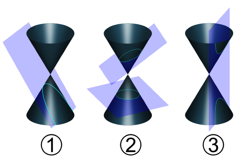
Figure 4. The Conic Sections: (1) Parabola, (2) Ellipse and Circle, (3) Hyperbola. (This image is in the public domain.)
If the plane intersects the vertex of the cone, then the result will be one of three "degenerate" cases: a pair of intersecting lines, a single line, or a single point.
The conic sections were first studied by mathematicians of ancient Greece. Pappus credited Euclid with writing four volumes on conic sections (which have been lost to history), and Apollonius with completing these volumes and writing an additional four. In Conics, Apollonius proved that two (distinct, nondegenerate) conic sections intersect in at most four points [Katz 2008, p. 122]. Therefore, four points do not uniquely determine a conic section, as illustrated in the applet in Figure 5.
Figure 5. Multiple conics passing through four points. Move points \(A,B,C,\) and \(D\) to explore the possibilities. (Interactive applet created using GeoGebra.)
When Nine Points Are Worth But Eight: Euler’s Resolution of Cramer’s Paradox - Construction of Conics
There are various constructions of particular conic sections, such as Euclid's Proposition IV.5, but a geometric construction of an arbitrary conic given five points was first published by William Braikenridge [1733], although Maclaurin disputed his priority in "a rather disagreeable controversy" [Coxeter 1961a, p. 91]. Coxeter gave the construction in both [1961a, p. 91] and [1961b, p. 254]. He suggested that it was based on Pascal's celebrated theorem about the points of intersection of the sides of a hexagon inscribed in a conic section. However, it is not clear that either Maclaurin or Braikenridge knew Pascal's Theorem; see [Mills 1984]. The applet in Figure 6 illustrates that, in general, there exists a conic section passing through any five points.
Figure 6. A conic section passing through five points. Move points \(A,B,C,D,\) and \(E\) to explore the possibilities. (Interactive applet created using GeoGebra.)
When Nine Points Are Worth But Eight: Euler’s Resolution of Cramer’s Paradox - Equations of Conics
In the 17th century, when analytic geometry was a brand new subject, mathematicians discovered that each of the conic sections may be expressed algebraically with an equation in the standard form \[\alpha y^2 + \beta xy + \gamma x^2 + \delta y + \varepsilon x + \zeta = 0.\]
For example, the equation of the circle \[(x - h)^2 + (y - k)^2 = r^2\] can be expanded and then expressed in the standard form above, with
| \(\alpha = 1,\) | \(\beta = 0,\) | \(\gamma = 1,\) |
| \(\delta = -2k,\) | \(\varepsilon = -2h,\) | \(\zeta = h^2 + k^2 - r^2.\) |
Similarly, the equation of the parabola \(y = ax^2 + bx + c\) can be expressed in standard form, where
| \(\alpha = 0,\) | \(\beta = 0,\) | \(\gamma = a,\) |
| \(\delta = -1,\) | \(\varepsilon = b,\) | \(\zeta = c.\) |
Furthermore, the type of conic section represented by an equation in standard form may be readily deduced from the coefficients of the equation. To do so, one first calculates the quantity \(\Delta=\beta^2 - 4 \alpha \gamma,\) known as the discriminant of the equation.
- When \(\Delta > 0,\) the curve is a hyperbola.
- When \(\Delta = 0,\) the curve is a parabola.
- When \(\Delta < 0,\) the curve is an ellipse (and if also \(\alpha=\gamma\) and \(\beta = 0,\) then the ellipse is a circle).
In general, given 5 points on a conic section, we can find the corresponding equation of degree 2 in a way that is similar to the way we found the equation of a parabola in an earlier section. We substitute the values \((x_1, y_1),\) \((x_2, y_2),\) \((x_3, y_3),\) \((x_4, y_4),\) and \((x_5, y_5)\) into the equation \[\alpha y^2 + \beta xy + \gamma x^2 + \delta y + \varepsilon x + \zeta = 0.\] As before, we obtain a system of linear equations in the variables \(\alpha, \beta, \gamma, \delta, \varepsilon, \zeta.\) Then, provided that certain algebraic conditions regarding the points are satisfied, a unique solution can be found. As with the cases of the circle and the parabola, these algebraic conditions concern the collinearity of the points under consideration. These conditions were investigated by Euler, as we will see in the sections that follow.
When Nine Points Are Worth But Eight: Euler’s Resolution of Cramer’s Paradox - Conic Exceptions
Leonhard Euler wrote a letter to Gabriel Cramer on October 20, 1744. Although all of Euler's other letters to Cramer were preserved in an archive in Geneva, Switzerland, this particular one went missing long ago and was unknown when scholars compiled a catalog of Euler's correspondence [Euler 1975]. The lost letter became known to Euler scholars at the meeting of the Euler Society in August 2003, which both authors of this article attended. At some point in the 20th century, it had found its way into the private collection of Bern Dibner (1897-1988). Dibner was an engineer, entrepreneur and philanthropist, as well as a historian of science. Over the course of his long life, he amassed an impressive private collection of rare books, manuscripts and letters. He donated about a quarter of this collection to the Smithsonian Library in 1974 and Euler's lost letter to Cramer was part of that gift. Mary Lynn Doan, professor of mathematics at Victor Valley College, had contacted the Dibner Library of the Smithsonian Institution in the summer of 2003 and learned that it has a small collection of documents by Leonhard Euler from Dibner's collection [Euler Papers]. She brought a photocopy of the letter with her to the Euler Society's meeting that summer and one of the authors (Bradley) was able to identify the addressee as Cramer. Shortly afterwards, he brought the letter to the attention of Andreas Kleinert, one of the editors of Euler's Opera Omnia [Euler]. The letter, in its original French, will appear in a forthcoming volume of Euler's correspondence.
In his letter to Cramer, Euler observed that there are exceptions to the rule that five points determine a conic section [Euler 1744b, p. 3]:
We may clarify this ... by considering lines of the second order, for the determination of which 5 points may not always be sufficient. For when all the five points are arranged on a straight line so that they give, for example, these equations
all of the coefficients of the general equation \(\alpha yy + \beta xy + \gamma xx + \delta y + \varepsilon x + \zeta = 0\) will not be determined, for after having introduced all of the given determinations, we are brought to this equation \(\alpha yy - (\alpha + \gamma)xy + \gamma xx + \delta y - \delta x = 0,\) so that there still remain two coefficents to be determined. If from the five given points there had been but 4 arranged in a straight line, then there would remain but one coefficient to be determined.
\(x=0;\)
\(y=0;\)\(x=1;\)
\(y=1;\)\(x=2;\)
\(y=2;\)\(x=3;\)
\(y=3;\)\(x=4;\)
\(y=4;\)
Euler did not use ordered pairs as we do today, but he was asking Cramer to consider the problem of trying to fit the points \((0,0),\) \((1,1),\) \((2,2),\) \((3,3)\) and \((4,4)\) to the general equation of the second degree, \[\alpha y^2 + \beta xy + \gamma x^2 + \delta y + \varepsilon x + \zeta = 0.\] (It's interesting to note that Euler wrote \(yy\) and \(xx\) where we would write \(y^2\) and \(x^2.\)) In this case, it turns out there is no unique solution to this equation.
When Nine Points Are Worth But Eight: Euler’s Resolution of Cramer’s Paradox - Five in a Row
Euler did not use matrices as we might today to find the coefficients in the general second degree equation \[\alpha y^2 + \beta xy + \gamma x^2 + \delta y + \varepsilon x + \zeta = 0.\] He simply substituted values and manipulated equations. Substituting \(x=y=0\) into the equation gives \(\zeta=0.\) The points \((1,1)\) and \((2,2)\) give rise to the equations
| \(\alpha + \beta + \gamma + \delta + \varepsilon\) | \(=0\) |
| \(4\alpha + 4\beta + 4\gamma + 2\delta + 2\varepsilon\) | \(=0.\) |
These can be simplified to
| \(\alpha + \beta + \gamma\) | \(=0\) |
| \(\delta + \varepsilon\) | \(=0,\) |
which in turn give \(\beta = -(\alpha + \gamma)\) and \(\varepsilon = -\delta.\) Substituting these back into the general equation \[\alpha y^2 + \beta xy + \gamma x^2 + \delta y + \varepsilon x + \zeta = 0\] gives us \[\alpha y^2 - (\alpha + \gamma)xy + \gamma x^2+\delta y - \delta x = 0,\] as Euler observed in his letter. The problem is that when \((3,3)\) or \((4,4)\) (or any point of the form \((k,k)\)) is substituted in this equation, the result is \(0=0.\) Thus, in modern terms, the five points \((0,0),\) \((1,1),\) \((2,2),\) \((3,3)\) and \((4,4)\) give rise to a system only of rank 3, and there is no unique solution.
The equation \[\alpha y^2 - (\alpha + \gamma)xy + \gamma x^2 +\delta y - \delta x = 0\] can be factored as
\[(y-x)(\alpha y - \gamma x + \delta) = 0.\]
Because a product can only be zero if one of its factors is zero, this in turn means that \[y-x=0 \quad\mbox{or} \quad \alpha y -\gamma x + \delta=0.\]
The first of these equations is the equation of the line \(y=x,\) which contains all of the given points. The other equation is a completely arbitrary linear equation, which could even be \(y=x.\) As long as \(\alpha\ne 0,\) it can be re-written as \[y = mx + b, \quad\mbox{where} \quad m = \frac{\gamma}{\alpha}\quad \mbox{and} \quad b = -\frac{\delta}{\alpha}.\]
This slope and intercept can be thought of as the "two coefficients to be determined" that Euler mentioned and the factored equation \[(y-x)(\alpha y - \gamma x + \delta) = 0\] becomes \[(y-x)(y-mx-b)=0.\]
We note that if \(\alpha = 0\) in the factored equation \[(y-x)(\alpha y - \gamma x + \delta) = 0,\] then the second equation is of a vertical line. In this case, the two coefficients in question are \(\alpha = 0,\) and the \(x\)-value \({\delta}/{\gamma}.\)
When Nine Points Are Worth But Eight: Euler’s Resolution of Cramer’s Paradox - Three or Four in a Row
Euler also considered the possibility of only four points in a line. For example, given the points \((0,0),\) \((1,1),\) \((2,2),\) \((3,3)\) and \((4,4),\) we might replace \((4,4)\) with some point \(A\) not on the line \(y=x.\) Let's suppose that \(A\) is \((1,2),\) for example, and substitute those values into the equation \[(y-x)(\alpha y - \gamma x + \delta) = 0\] from the preceding section. This will give us \(2\alpha - \gamma + \delta = 0.\) If we solve this equation for \(\delta\) and substitute it into \(\alpha y - \gamma x + \delta=0,\) we get \[y = mx + (2-m), \quad \mbox{where} \quad m = \frac{\gamma}{\alpha}.\]
This is the equation of a line with arbitrary slope \(m\) and intercept \(b=2-m,\) so that it passes through the point \((1,2).\) As Euler said, there is "one coefficient to be determined," which we can think of as the slope of the line. We observe that we could also have determined this equation by substituting the point \((1,2)\) into the equation \[(y-x)(y - mx - b) = 0.\]
Finally, let's consider a case that Euler didn't mention but was certainly familiar with: the case of three points in a line. In this case, the coefficients are all determined, but the graph of the equation is still exceptional.
Figure 7. A degenerate, two-line conic section. Move points \(A\) and \(B\) to explore the possibilities. (Interactive applet created using GeoGebra.)
Given the points \((0,0),\) \((1,1),\) \((2,2),\) \((3,3)\) and \((1,2),\) we replace the point \((3,3)\) with another point \(B\) not on the line \(y=x.\) Let's use the point \((2,1)\) as an example; in the applet in Figure 7 above, \(B\) can be any point at all. If we substitute \((2,1)\) into the equation \[(y-x)(y - mx - b) = 0,\] we get \(b=1-2m.\) But because we already know that that \(b=2-m,\) we have \(m=-1,\) which is the slope of the line passing through \((1,2)\) and \((2,1).\) This means that the equation \[(y-x)(y - mx - b) = 0\] becomes \[(y−x)(y+x−3)=0,\] whose graph is the union of the graphs of the lines \(y=x\) and \(y=-x+3.\)
This situation is an important case of the degenerate conic. Whenever we have three collinear points and two other points not on that line, then the equation of the conic is always uniquely determined, up to a multiplicative factor, but it is an equation that can be factored into a product of two linear equations, one of which is satisfied by the three collinear points, the other of which is satisfied by the two additional points. Probably the most familiar example of a degenerate conic has the equation \(y^2-x^2=0,\) which factors as \((y-x)(y+x)=0.\) However, if four or five points are collinear, then the equation has an undetermined linear factor and there are infinitely many conic sections passing through the given points.
When Nine Points Are Worth But Eight: Euler’s Resolution of Cramer’s Paradox - Higher Order Equations
Now that we understand the relationship between a second order equation and the various kinds of conic sections, let's turn our attention to equations of higher order. A polynomial equation in two variables is an equation of the form \[p(x,y)=0,\] where \(p(x,y)\) is a polynomial. The terms of \(p(x,y)\) have the form \(c x^i y^j,\) where \(c\) is a constant coefficient and \(i\) and \(j\) are non-negative integers. We assume that \(p(x,y)\) has been simplified so that there is only one such term for any particular pair \(i\) and \(j.\) The degree of the term \(c x^i y^j\) is \(i+j.\) Clearly, there can only be one term of degree 0, two terms of degree 1 and, in general, \(n+1\) terms of degree \(n.\)
The degree of a polynomial equation of the form \(p(x,y)=0\) is the maximum of the degrees of the terms of \(p(x,y).\) Therefore, the general form of a polynomial equation of degree one (a linear equation) is
\[A x + B y + C = 0.\]
The general form of a polynomial equation of degree two (a quadratic equation) was written by Euler as
\[\alpha y^2 + \beta xy + \gamma x^2 + \delta y + \varepsilon x + \zeta = 0.\]
The general form of a polynomial equation of degree \(n\) is
\[\sum^{n}_{k=0} \sum^{k}_{i=0} \alpha_{k,i} x^i y^{k-i} = 0,\]
where the \(\alpha_{k,i}\) are constant coefficients and there is at least one \(i_0\) with \(0 \le i_0 \le n\) satisfying \(\alpha_{n,i_0} \ne 0.\) Using the familiar formula for the sum of the first \(N\) integers, the number of coefficients in a polynomial equation of degree \(n\) is the sum \[1 + 2 + 3 + \ldots + n + (n+1) = \frac{(n+1)(n+2)}{2} = \frac{n^2+3n}{2} + 1.\]
A curve of degree \(n\) (called a "line" of degree \(n\) by Euler and most other 18th century authors) is the graph of the solution set of a polynomial equation of degree \(n.\) An equation of the form \(p(x,y)=0\) may be multiplied by an arbitrary non-zero constant without changing the set of pairs \((x,y)\) that satisfy it. Therefore, in order to determine its solution set, it's only necessary to specify the ratios among the coefficients of \(p(x,y),\) not the coefficients themselves. The number of such ratios, denoted \(\varphi_n,\) is one less than the number of coefficients; that is \[\varphi_n = \frac{n^2+3n}{2}.\]
When Nine Points Are Worth But Eight: Euler’s Resolution of Cramer’s Paradox - Determination of Higher Order Curves
Cramer is usually given credit for the result that \(\frac{n^2+3n}{2}\) points generally determine a curve of degree \(n,\) because he gave a proof of it, using the counting argument on the preceding page, in Chapter 3 of his book Introduction a l'analyse des lignes courbes algébriques (Introduction to the Analysis of Curved Algebraic Lines) [Cramer 1750], which was widely read in the second half of the 18th century. Euler proved the same thing in a paper published in the same year [Euler 1750a], but the result had actually been published much earlier by Maclaurin [Maclaurin 1720].
To determine a curve of degree \(n,\) it is usually enough to know \(\varphi_n = \frac{n^2+3n}{2}\) points that lie on the curve. These will give rise to a homogeneous system of \(\varphi_n\) equations in \(\varphi_n + 1\) unknowns. As long as the rank of this system is \(\varphi_n,\) then the \(\varphi_n + 1\) coefficients of the polynomial equation will be determined, up to a scalar multiple. However, as Euler's example indicates, the linear equations may not be linearly independent for every possible set of \(\varphi_n\) points on the curve. In particular, a conic should be determined by \(\varphi_2=5\) of its points, but not when 4 or 5 of the points lie on the same line.
Let's consider the case of the cubic equation, i.e. the polynomial equation of degree 3. In [Euler 1750a], Euler wrote the general cubic equation as
\[\alpha x^3 + \beta x^2y + \gamma xy^2 + \delta y^3 + \varepsilon x^2 + \zeta xy + \eta y^2 + \theta x + \iota y + \kappa = 0.\]
If we now substitute \((x_1,y_1),\) \((x_2,y_2),\) …, \((x_9,y_9),\) we have a system of 9 equations in the 10 unknowns \(\alpha,\) \(\beta,\) …, \(\kappa,\) represented by the following augmented matrix:\[\left[\begin{array}{rrrrrrrrrrr} x_1^3 & x_1^2y_1 & x_1y_1^2 & y_1^3 & x_1^2 & x_1y_1 & y_1^2 & x_1 & y_1 & 1 & 0 \\ x_2^3 & x_2^2y_2 & x_2y_2^2 & y_2^3 & x_2^2 & x_2y_2 & y_2^2 & x_2 & y_2 & 1 & 0 \\ x_3^3 & x_3^2y_3 & x_3y_3^2 & y_3^3 & x_3^2 & x_3y_3 & y_3^2 & x_3 & y_3 & 1 & 0 \\ x_4^3 & x_4^2y_4 & x_4y_4^2 & y_4^3 & x_4^2 & x_4y_4 & y_4^2 & x_4 & y_4 & 1 & 0 \\ x_5^3 & x_5^2y_5 & x_5y_5^2 & y_5^3 & x_5^2 & x_5y_5 & y_5^2 & x_5 & y_5 & 1 & 0 \\ x_6^3 & x_6^2y_6 & x_6y_6^2 & y_6^3 & x_6^2 & x_6y_6 & y_6^2 & x_6 & y_6 & 1 & 0 \\ x_7^3 & x_7^2y_7 & x_7y_7^2 & y_7^3 & x_7^2 & x_7y_7 & y_7^2 & x_7 & y_7 & 1 & 0 \\ x_8^3 & x_8^2y_8 & x_8y_8^2 & y_8^3 & x_8^2 & x_8y_8 & y_8^2 & x_8 & y_8 & 1 & 0 \\ x_9^3 & x_9^2y_9 & x_9y_9^2 & y_9^3 & x_9^2 & x_9y_9 & y_9^2 & x_9 & y_9 & 1 & 0\end{array}\right].\]
For example, the entries in the second column are the numbers \(x_i^2y_i,\) because the second unknown coefficient (\(\beta\)) is the coefficient of \(x^2y.\)
Suppose that we apply elementary operations to put this matrix into a reduced row-echelon form. If the rank of the system is 9, then there will be infinitely many solutions depending on one parameter, say \(t.\) Because the system is homogeneous, we will always be able to solve for the non-zero coefficients as multiples of \(t.\) This will give us a unique solution of the general cubic equation \[\alpha x^3 + \beta x^2y + \gamma xy^2 + \delta y^3 + \varepsilon x^2 + \zeta xy + \eta y^2 + \theta x + \iota y + \kappa = 0\] up to an arbitrary factor \(t\) on the left-hand side. However, if the rank of the system is less than 9, then the general cubic equation will not be determined up to scalar multiplicity.
When Nine Points Are Worth But Eight: Euler’s Resolution of Cramer’s Paradox - Cramer's Paradox
Now let's suppose we have two cubic equations that are not multiples of one another. By Bézout's Theorem, it's possible for their curves to intersect in 9 points. Maclaurin, Cramer and Euler were all perplexed by this situation, because they knew the counting argument that shows that 9 points should generally give a unique curve of degree 3. The situation is even worse for \(n > 3.\) For example, two curves of degree \(n=4\) can intersect in \(n^2=16\) places and yet 14 points should suffice to determine such a curve uniquely. Here's what Maclaurin wrote about it (see [Maclaurin 1720, p. 137] or [Scott 1898, p. 260]):
A line of order \(n\) may intersect another of the same order in \(n^2\) points. Accordingly, when two lines of order \(n\) pass through \(n^2\) points, the given points, of which the number is \(\frac{1}{2}(n^2+3n),\) are not sufficient for determining the line of order \(n\) whose curve would be the unique curve that passes through the given points. … Thus, if nine points don't sufficiently determine a line of the third order, … nevertheless, 10 are more than enough for determining a line of the third order.
Maclaurin apparently could not resolve the paradox, but it did not cause him to abandon the proposition that \(\frac{1}{2}(n^2+3n)\) points determine a curve of order \(n.\) This was not the case for Braikenridge. Because he knew that two curves of degree \(n\) could intersect in \(n^2\) points, he concluded that the number of points needed to determine such a curve uniquely had to be greater than \(n^2.\) In [Braikenridge 1735], he argued that the number of points needed was \(n^2+1.\)
Cramer read Braikenridge's article and brought it to Euler's attention in a letter of 30 September 1744, the letter that preceded [Euler 1744b] in their correspondence. Cramer did not mention Maclaurin's argument in his letter to Euler, but Euler replied as follows [Euler 1744b, p. 2]:
I have seen that Mr. Maclaurin already had the same doubt concerning the number of points which determine curves of a given order: he says that to determine a line of the third order, the number of nine points may be too small, yet still the number of ten is too great, which in my opinion is an overt contradiction. The aforementioned Braikenridge is also absolutely mistaken in holding that a line of order \(n\) may be described by \(n^2+1\) points and it is a disputed truth, as you have very well remarked, that this number is but \(\frac{nn+3n}{2}.\) Furthermore, one may not doubt that two curved lines, one of which is of order \(m\) and the other of order \(n,\) may intersect in \(mn\) points, though you will be the first to have given a perfect proof of this truth, for I freely admit that my proof is all but complete.
It is interesting to note the status of Bézout's Theorem in 1744. Cramer had told Euler that he had a proof of it, which would soon appear in his book [Cramer 1750]. It would actually take six years for the book to be published. Meanwhile, Euler figured that he had just proved it himself, more or less, so that Cramer would still be the first to publish. It turned out that neither Euler's proof (in [Euler 1750b]) nor Cramer's were considered complete, so the theorem remained an open conjecture for another generation to tackle.
Euler continued in his letter to Cramer as follows [Euler 1744b, p. 2]:
At first, all of these reflections only served to bring to my attention the difficulties of the case, which you were so good as to propose to me. However, I finally found the solution to this doubt, with which I hope you will be satisfied. I say, then, that although it is indeed true that a line of order \(n\) be determined by \(\frac{nn+3n}{2}\) points, this rule is nevertheless subject to certain exceptions. For although the general equation of lines of order \(n\) has \(\frac{nn+3n}{2}\) coefficients to be determined, it may happen that such a number of equations, which we draw from the same number of given points, is not sufficient for this effect: this is evident, when two or several of these equations become identical. In such a case, one finds after having reduced the matter to the determination of the final coefficient, the value of this is expressed by a fraction, whose numerator and denominator both become =0. I conceive therefore, that this inconvenience will take place when the nine points, which ought to determine a line of the 3rd order, are disposed such that two curved lines of this order may be drawn through them. In this case, the nine given points, since they contain two identical equations, are worth but 8, and we may then add the tenth point in order to render the problem determined.
Euler did not have the language of linear independence and rank, but his resolution of the paradox can be expressed as follows: if we choose 9 points on a cubic curve that happen to be the same 9 points where that curve intersects a different cubic curve, then that collection of points is not suitably "generic" and it gives rise to a system of 9 equations in 10 unknowns with a rank of only 8. In this case, there will be two parameters in the solution space, so the solutions, which give the coefficients of the general cubic equation \[\alpha x^3 + \beta x^2y + \gamma xy^2 + \delta y^3 + \varepsilon x^2 + \zeta xy + \eta y^2 + \theta x + \iota y + \kappa = 0,\] will not all be scalar multiples of one another. When this happens, there really will be infinitely many distinct cubic curves passing through the 9 given points.
Working in the 18th century, Euler had neither the definitions nor the results of linear algebra at his disposal, so a proof of this assertion was beyond his means (see [Dorier 1995] for more on the state of vector space theory in the 1700s). In his letter to Cramer, he could not even give a concrete example of a set of 9 points with the property that infinitely many cubic curves pass through them. Instead, he had to be content with arguing by analogy with the case where 5 points do not determine a unique conic when 4 or more of them lie in a straight line. However, it would not be long before Euler came up with a beautiful example to illustrate the correctness of his claim.
When Nine Points Are Worth But Eight: Euler’s Resolution of Cramer’s Paradox - Euler's Elegant Example
In the fall of 1747, Euler read a paper to the Berlin Academy titled "On an apparent contradiction in the theory of curved lines." It was published soon afterwards [Euler 1750a], coincidentally in the same year that Cramer published his book on the analysis of curved lines [Cramer 1750]. In this paper, Euler carefully explained Cramer's Paradox and gave examples of various linear systems in which one or more of the given equations is "contained in the others" – in modern terms, where one or more equation is a linear combination of the remaining equations, so that the rank of the system is less that the number of equations. He then described his resolution of Cramer's paradox and closed with examples of sets of nine points that do not uniquely determine a cubic curve. Most of his examples are degenerate cubics whose equation can be factored as the product of an equation of order two and another of order one, or as a product of three linear equations. Cubic curves such as these generally consist either of a straight line and a conic section, or of three straight lines.
Euler's pièce de resistance was the example consisting of 9 points arranged in a \(3 \times 3\) square grid. For simplicity, let's assume these are the points \((0,0),\) \((1,0),\) \((0,1),\) \((-1,0),\) \((0,-1),\) \((1,1),\) \((-1,1),\) \((-1,-1)\) and \((1,-1)\) (Euler considered the slightly more general case with \(\pm a\) replacing \(\pm 1,\) for an arbitrary constant \(a>0\)). We can try to fit a cubic equation through these points by substituting the \(x\)- and \(y\)-coordinate of each point into the general cubic equation
\[\alpha x^3 + \beta x^2y + \gamma xy^2 + \delta y^3 + \varepsilon x^2 + \zeta xy + \eta y^2 + \theta x + \iota y + \kappa = 0,\]
and setting up a system of 9 linear equations in the 10 unknown coefficients of this equation.
A modern brute force method of doing this might begin with the homogeneous augmented matrix \[\left[\begin{array}{rrrrrrrrrrr} 0 & 0 & 0 & 0 & 0 & 0 & 0 & 0 & 0 & 1 & 0 \\1 & 0 & 0 & 0 & 1 & 0 & 0 & 1 & 0 & 1 & 0 \\0 & 0 & 0 & 1 & 0 & 0 & 1 & 0 & 1 & 1 & 0 \\-1 & 0 & 0 & 0 & 1 & 0 & 0 &-1 & 0 & 1 & 0 \\0 & 0 & 0 &-1 & 0 & 0 & 1 & 0 &-1 & 1 & 0 \\1 & 1 & 1 & 1 & 1 & 1 & 1 & 1 & 1 & 1 & 0 \\-1 & 1 &-1 & 1 & 1 &-1 & 1 &-1 & 1 & 1 & 0 \\-1 &-1 &-1 &-1 & 1 & 1 & 1 &-1 &-1 & 1 & 0 \\1 &-1 & 1 &-1 & 1 &-1 & 1 & 1 &-1 & 1 & 0 \\ \end{array}\right].\]
We would then apply elementary matrix operations to transform it into the reduced row-echelon form \[\left[\begin{array}{rrrrrrrrrrr}1 & 0 & 0 & 0 & 0 & 0 & 0 &1 & 0 & 0 & 0 \\0 & 1 & 0 & 0 & 0 & 0 & 0 & 0 & 0 & 0 & 0 \\0 & 0 & 1 & 0 & 0 & 0 & 0 & 0 & 0 & 0 & 0 \\0 & 0 & 0 & 1 & 0 & 0 & 0 & 0 &1 & 0 & 0 \\0 & 0 & 0 & 0 & 1 & 0 & 0 & 0 & 0 & 0 & 0 \\0 & 0 & 0 & 0 & 0 & 1 & 0 & 0 & 0 & 0 & 0 \\0 & 0 & 0 & 0 & 0 & 0 & 1 & 0 & 0 & 0 & 0 \\0 & 0 & 0 & 0 & 0 & 0 & 0 & 0 & 0 & 1 & 0 \\0 & 0 & 0 & 0 & 0 & 0 & 0 & 0 & 0 & 0 & 0 \\\end{array}\right].\]
If we let \(\theta = s\) and \(\iota = -t\) for arbitrary real numbers \(s\) and \(t,\) then \(\alpha = -s,\) \(\delta = t,\) and the general cubic equation \[\alpha x^3 + \beta x^2y + \gamma xy^2 + \delta y^3 + \varepsilon x^2 + \zeta xy + \eta y^2 + \theta x + \iota y + \kappa = 0\] becomes \[-s x^3 + t y^3 + sx - ty = 0,\] or \[t(y^3-y) = s(x^3-x).\]
Euler simply gave the solution, which he wrote as \(my(yy-aa)=nx(xx-aa),\) and left the details to the reader. His solution process was probably something like the following. We first consider \((0,0),\) which gives \(\kappa = 0.\) Next, the points \((\pm 1,0)\) give us the equations \[\alpha + \varepsilon + \theta = 0\]\[-\alpha + \varepsilon - \theta = 0,\] which are equivalent to the equations \(\varepsilon = 0\) and \(\alpha + \theta = 0.\) Similarly, the points \((0,\pm 1)\) give us \(\eta = 0\) and \(\delta + \iota = 0.\) Therefore, the general cubic equation \[\alpha x^3 + \beta x^2y + \gamma xy^2 + \delta y^3 + \varepsilon x^2 + \zeta xy + \eta y^2 + \theta x + \iota y + \kappa = 0\] reduces to \[\alpha(x^3-x) + \beta x^2y + \gamma xy^2 + \delta(y^3-y) + \zeta xy = 0.\] If we substitute the points \((1,1),\) \((-1,1)\) and \((1,-1),\) respectively, we have \[\begin{array}{rrr}\beta + \gamma + \zeta &=& 0\\ \beta - \gamma - \zeta &=& 0\\-\beta + \gamma - \zeta &=& 0.\end{array}\]
From these we deduce \(\beta = \gamma = \zeta = 0\) or \[\alpha(x^3-x) + \delta(y^3-y) = 0.\]
Because the point \((-1,-1),\) which we have not used yet, yields \(0=0\) when substituted, the system has rank 8 or, as Euler put it in his letter to Cramer, the nine points “are worth but 8.”
When Nine Points Are Worth But Eight: Euler’s Resolution of Cramer’s Paradox - An Infinite Family of Curves
Consider the cubic equation for Euler's Elegant Example: \[ t(y^3-y) = s(x^3-x).\]
As long as \(t \ne 0,\) we can divide through by \(t.\) If we then let \(p={s}/{t},\) we have the parameterized cubic equation \[ y^3-y = p(x^3-x).\]
Now for any real number that we assign to the parameter \(p,\) we have an equation whose graph passes through the nine points of the \(3 \times 3\) grid. You can explore these curves using the applet in Figure 8. You can set particular values of \(p\) using the slider control, or put the applet into play mode and watch as \(p\) cycles through values between \(-4\) and \(+4.\)
Figure 8. Euler's Elegant Example. Set values of \(p\) using the slider control, or click the arrow at lower left and watch as \(p\) cycles through values between \(-4\) and \(+4.\) (Interactive applet created using GeoGebra.)
For the particular values \(p=0,\, p=1,\) and \(p=−1,\) we can factor the parameterized cubic equation \[ y^3-y = p(x^3-x)\] into factors of lower order.
|
Value of \(p\) |
Factorization |
|
\(−1\) |
\((y+x)(y^2−xy+x^2−1)=0\) |
|
\(0\) |
\(y(y−1)(y+1)=0\) |
|
\(1\) |
\((y−x)(y^2+xy+x^2−1)=0\) |
There is one more important special case, when \(t=0\) in the original equation \[t(y^3-y) = s(x^3-x)\] for Euler's Elegant Example. In this case, we have \(x(x-1)(x+1) = 0,\) so that the graph consists of three vertical lines: \(x=0,\) \(x=1\) and \(x=-1.\) This is the asymptotic case to which the parameterized cubic equation \[ y^3-y = p(x^3-x)\] tends when either \(p \rightarrow +\infty\) or \(p \rightarrow -\infty.\)
When Nine Points Are Worth But Eight: Euler’s Resolution of Cramer’s Paradox - Euler's Resolution Vindicated
After describing his beautiful example, Euler wrote these words [Euler 1750a, p. 232]:
And from this one will easily understand that every time that two curves of the third order intersect at 9 points, these points will be such that they do not completely determine a curve of the third order, and that in the general equation, after one had applied it to these nine points, a coefficient will remain undetermined. In these cases, therefore, there will be not only two curves of the third order, but an infinity of curves of this order, which can all be described by these nine points.
A modern reader might reasonably object that Euler had not proved the general claim he made in this passage. Rather, having given an illustrative example, he simply asked the reader to understand – or perhaps simply to accept – that the general case was similar. However, Charlotte Scott [1898, p. 263] pointed to this very passage as an indication that Euler's explanation of Cramer's Paradox went "just a little bit further" than the one that Cramer himself gave in [Cramer 1750]. Further reading on Euler's contribution to the resolution of Cramer's Paradox can be found in [Sandifer 2007].
An entirely satisfactory resolution of Cramer's Paradox would have to wait until the 19th century, when the concepts of linear algebra were more well formed. In fact, nineteenth century mathematicians continued to work on generalizations and elaborations of Cramer's Paradox. For more on the further development of this problem, see the historical introduction to [Eisenbud 1996]. In particular, Michel Chasles (1793-1880) fully vindicated Euler's resolution of Cramer's Paradox for cubic curves; see [Eisenbud 1996, p. 301]. Arthur Cayley (1821-1895) worked on the higher degrees and proved the following theorem, as quoted in [Scott 1898]:
Theorem (Cayley 1843, parenthesized hypothesis added 1887). Suppose \(n \ge l,\) \(n \ge m,\) \(n < l+m,\) and let \[\delta = \frac{1}{2}(l+m-n-1)(l+m-n-2).\] If a curve of order \(n\) passes through \(lm-\delta\) of the points of intersection of two curves of order \(l\) and \(m,\) then it necessarily passes through the remaining \(\delta\) points (unless those \(\delta\) points lie on a curve of order \(l+m-n-3\)).
Euler's example is indeed generic: in the case \(l=m=n=3,\) Cayley's theorem says that a curve of order 3 that passes through any 8 of the 9 points of intersection of two curves of order 3 must necessarily pass through all 9. Thus, the rank of the linear system determined by these 9 points can't possibly be more than 8. In the more general case of Cramer's Paradox, if \(l=m=n \ge 3,\) then Cayley's theorem says that a curve of order \(n\) passing through any \(\frac{n^2+3n}{2}-1\) of the \(n^2\) points of intersection of two curves of order \(n\) necessarily passes through all \(n^2\) points, unless those remaining points all lie on a curve of order \(n-3.\)
When Nine Points Are Worth But Eight: Euler’s Resolution of Cramer’s Paradox - Euler's Letter to Cramer
The full text of Euler's letter to Cramer of October 20, 1774 is reproduced here in English translation.
Sir,
As I have not yet seen my work, which has just come off the press,1 I am infinitely obliged to you for the particular trouble you have taken with the corrections. But great though my obligation to you may be, so much greater should be my sympathy for the precious time you have expended, and the scientific community [les Scavans] should be very displeased with me for causing you to have turned away from your usual occupations, so highly esteemed by all. It is because of this consideration that I completely approve of the reply you have made to Mr. Bousquet, in refusing your assistance with respect to proofreading my work,2 which he wishes to publish, not doubting for a moment that he would never find a man as qualified for the task as you in Lausanne. I have learned with great pleasure that you have composed a piece on the same material3 and, as I am extremely curious to see it, I add my wishes to those of Mr. Bousquet to encourage you to publish it. In my opinion, these matters have, by and large, not yet been properly explained and I do not doubt that you have clarified a great number of situations that have eluded me, as well as others who have written on the subject. One finds there questions so thorny, that one must apply to them all possible attention so as not to fall into error, as happened to me in my explanation of the cuspidal point of the second kind.4 Mr. the Marquis de l'Hopital showed that there are in fact curves endowed with such a point,5 but Mr. Gua de Malves holds that the two branches of a curve which form the point always extend to the other side so that, according to him, this point is nothing but the intersection of two branches, which cross in an infinitely small angle.6 These arguments convinced me that he was right, as you no doubt noted in looking over my work. But since then, I have recognized quite clearly that I was mistaken on this and that there actually are curves that have such a cusp point by itself, one that cannot be regarded as the infinitely close intersection of two branches. Even in the fourth order there is a curved line of this kind, whose equation is7 \[y^4 - 2xy^2 + xx = x^3 + 4yxx,\] which simplifies to \[y=\sqrt{x} \pm \sqrt[4]{x^3}.\]
The reason I was mistaken is that I believed that this curve ought to have a diameter,8 since \(\sqrt{x}\) may take a negative value as well as positive, but since the other term \(\sqrt[4]{x^3}\) is equal to the first one, \(\sqrt{x},\) multiplied by its own square root \(\sqrt{\sqrt{x}},\) one sees clearly we may not take the first \(\sqrt{x}\) to be negative, without the other \(\sqrt[4]{x^3}\) becoming imaginary. And in fact, if we give the \(\sqrt{x}\) term the \(-\) sign, then the equation
\[y=-\sqrt{x} \pm \sqrt[4]{x^3}\]
is resolved as
\[y^4 - 2xy^2 + xx = x^3 - 4yxx,\]
which is not the same curve in the same position. As I do not have a copy of my manuscript here, I beg you to add a little note at this location, if you have not already returned home.
I have seen that Mr. Maclaurin already had the same doubt concerning the number of points which determine curves of a given order: he says that to determine a line of the third order, the number of nine points may be too small, yet still the number of ten is too great, which in my opinion is an overt contradiction. The afore-mentioned Braikenridge is also absolutely mistaken in holding that a line of order \(n\) may be described by \(n^2+1\) points and it is a disputed truth, as you have very well remarked, that this number is but \(\frac{nn+3n}{2}.\) Furthermore, one may not doubt that two curved lines, one of which is of order \(m\) and the other of order \(n,\) may intersect in \(mn\) points, though you will be the first to have given a perfect proof of this truth, for I freely admit that my proof is all but complete. At first, all of these reflections only served to bring to my attention the difficulties of the case, which you were so good as to propose to me. However, I finally found the solution to this doubt, with which I hope you will be satisfied. I say, then, that although it is indeed true that a line of order \(n\) be determined by \(\frac{nn+3n}{2}\) points, this rule is nevertheless subject to certain exceptions. For although the general equation of lines of order \(n\) has \(\frac{nn+3n}{2}\) coefficients to be determined, it may happen that such a number of equations, which we draw from the same number of given points, is not sufficient for this effect: this is evident, when two or several of these equations become identical. In such a case, one finds after having reduced the matter to the determination of the final coefficient, the value of this is expressed by a fraction, whose numerator and denominator both become \(=0.\) I conceive therefore, that this inconvenience will take place when the nine points, which ought to determine a line of the 3rd order, are disposed such that two curved lines of this order may be drawn through them. In this case, the nine given points, since they contain two identical equations, are worth but 8, and we may then add the tenth point in order to render the problem determined. We may clarify this article to our further satisfaction by considering lines of the second order, for the determination of which 5 points may not always be sufficient. For when all the five points are arranged on a straight line so that they give, for example, these equations9
|
\(x=0;\) \(y=0;\) |
\(x=1;\) \(y=1;\) |
\(x=2;\) \(y=2;\) |
\(x=3;\) \(y=3;\) |
\(x=4;\) \(y=4;\) |
all of the coefficients of the general equation \(\alpha yy + \beta xy + \gamma xx + \delta y + \epsilon x + \zeta = 0\) will not be determined, for after having introduced all of the given determinations, we are brought to this equation \(\alpha yy - (\alpha + \gamma)xy + \gamma xx + \delta y - \delta x = 0,\) so that there still remain two coefficients to be determined. If from the five given points there had been but 4 arranged in a straight line, then there would remain but one coefficient to be determined. From this, one easily understands that if the nine points, from which one ought to draw a line of the third order, are at the same time the intersections of two curved lines of this order, then, after having completed all of the calculations, there must remain in the general equation for this order an undetermined coefficient, and beginning from this case not only two, but an infinity of lines of the 3rd order may be drawn from the same nine points.
The use, which you have made of continued fractions in dioptrics is admirably beautiful and I am extremely obliged to you for the theorem, which you have communicated to me. I am charmed that you recognize, along with me, that this material is of great use in mathematics and that it is quite worthy of attention. It is not only arithmetic that can draw much profit from it, but also the integral calculus, as I made known in several pieces on this subject that I left in Petersburg, one of which10 has already been published in the ninth volume of the Comm.
It is already a long time since Mr. Bousquet wrote to tell me that you had the kindness to send me a copy of the Works of Mr. James Bernoulli, which was shipped here along with a quantity of books for Mr. Neaulme. But since this latter was not willing to accept the package, I have received nothing. Had it not been for this, I would not have failed to thank you infinitely. I am therefore embarrassed that I do not find myself in a position to show my gratitude except in words, but rest assured, that should an opportunity present itself for me to render you service, I will employ all of my energy to discharge my obligation. I have the honor of being, with the most perfect esteem,
Sir,
Your very humble and very obedient servant L. Euler
Berlin this 20 October 1744
Notes on the Translation of Euler's Letter to Cramer
1 Here Euler referred to Methodus inveniendi lineas curvas [Euler 1744a], published in Lausanne by Bousquet in 1744.
2 Here Euler referred to Introductio in analysin infinitorum [Euler 1748], published in Lausanne by Bousquet in 1748.
3 Cramer's Introduction a l'analyse des lignes courbes algébraique [Cramer 1750], published by Bousquet in 1750, and volume 2 of Euler's Introductio [Euler 1748] both dealt with the theory of equations.
4 For more on the cuspidal point of the second kind and the importance of the 4th degree equation that follows, see [Bradley 2006].
5 See [L'Hôpital 1696].
6 See [Gua de Malves 1740].
7 The four equations in this paragraph were actually written by Euler as in-line equations. We have set them as displayed equations for greater clarity.
8 That is, Euler thought the curve was symmetric about the \(x\)-axis.
9 In modern notation, Euler considered the points \((0,0), (1,1), (2,2), (3,3),\) and \((4,4).\)
10 Euler referred to E71, "De fractionibus continuis dissertatio," which was presented to the St. Petersburg Academy on March 7, 1737. However, volume 9 of the Commentarii academiae scientiarum imperialis Petropolitanae, for the year 1737, did not actually appear until 1744.
When Nine Points Are Worth But Eight: Euler’s Resolution of Cramer’s Paradox - References
- [Boyer 1956] Boyer, C. B., History of Analytic Geometry, New York: Scripta Mathematica, 1956. Reprinted New York: Dover, 2004.
- [Bradley 2006] Bradley, R. E., "The Curious Case of the Bird's Beak," International J. Math. Comp. Sci. 1 (2006), no. 2, pp. 243-268.
- [Braikenridge 1733] Braikenridge, W. Exercitato Geometrica de Descriptione Curvarum, London, 1733.
- [Braikenridge 1735] Braikenridge, W., "A General Method of Describing Curves, by the Intersection of Right-Lines; Moving about Points in a Given Plane. In a Letter to Dr. Hoadly, by the Rev. Mr. Braikenridge," Phil. Trans. 39 (1735), no. 436, pp. 25-36.
- [Coxeter 1961a] Coxeter, H. S. M., The Real Projective Plane, 2nd. ed., Cambridge: Cambridge University Press, 1961.
- [Coxeter 1961b] Coxeter, H. S. M., Introduction to Geometry, New York: Wiley, 1961.
- [Cramer 1750] Cramer, G., Introduction a l'analyse des lignes courbes algébriques, Geneva: Cramer frères, 1750.
- [Dorier 1995] Dorier, J.-L., "A general outline of the genesis of vector-space theory," Historia Mathematica 22, 1995, 227-261.
- [Eisenbud 1996] Eisenbud, D., Green, M., Harris, J., "Cayley-Bacharach Theorems and Conjectures," Bulletin AMS 33 (1996), 295-324.
- [Euler Papers] Euler, Leonhard, "Leonhard Euler Papers" (MSS 490A), Dibner Library of the History of Science and Technology, Smithsonian Institution Libraries.
- [Euler] Euler, L., Leonhardi Euleri Opera Omnia, multiple volumes, publication begun in 1911 and in progress, Leipzig: Teubner, Zürich: Orell-Füssli, Basel: Birkhäuser.
- [Euler 1744a] Euler, L,. Methodus inveniendi lineas curvas maximi minimive..., Lausanne: Bousquet, 1744. Also in [Euler], ser. I, vol. 24.
- [Euler 1744b] Euler, L., 1744/10/20, letter to G. Cramer, in Leonhard Euler Papers (MSS 490A), Dibner Library of the History of Science and Technology, Smithsonian Institution Libraries.
- [Euler 1748] Euler, L., Introductio in Analysin Infinitorum, 2 vols., Lausanne: Bousquet, 1748. Also in [Euler], ser. I, vols. 8-9.
- [Euler 1750a] Euler, L., "Sur un contradiction apparente dans la doctrine des lignes courbes," Mém. Berlin, IV (1748), 1750, 219-233. Also in [Euler], ser. I, vol. 26, 33-45.
- [Euler 1750b] Euler, L., "Démonstration sur le nombre des points, ou deux lignes des ordres quelconques peuvent se couper," Mém. Berlin, IV (1748), 1750, 234-248. Also in [Euler], ser. I, vol. 26, 46-59.
- [Euler 1751] Euler, L., "Sur le point de rebroussement de la seconde espece de M. le Marquis de l'Hôpital," Mém. Berlin, V (1749), 1751, 203-221. Also in [Euler], ser. I, vol. 27, 236-252.
- [Euler 1975] Euler, L., Opera Omnia, Series IVA, volume 1 (index of Euler's correspondence), eds. A. P. Juškevič, V. I. Smirnov, W. Habicht, Basel: Birkhäuser, 1975.
- [Euler 2015] Euler, L., Opera Omnia, Series IVA, volume 7 (correspondence of Euler with G. Cramer and 8 others), eds. S. Bodenmann, A. Kleinert, Basel: Birkhäuser, to appear in 2015.
- [Gua de Malves 1740] Gua de Malves, J. P. de, Usages de l'analyse de Descartes pour découvrir, sans le secours du Calcul Differentiel, les Propriétés, ou affectations principales des lingnes géometriques de tous les ordres, Paris: Briasson, 1740.
- [L'Hôpital 1696] L'Hôpital, G., Analyse des infiniment petits, pour l'intelligence des lignes courbes, Paris: l'Imprimerie royale, 1696.
- [Katz 2008] Katz, Victor J., A History of Mathematics, 3rd ed., Boston: Addison-Wesley, 2008.
- [Maclaurin 1720] Maclaurin, C., Geometrica Organica; Sive Descriptio Linearum Curvarum Universalis, London, 1720.
- [Mills 1984] Mills, S. "Note on the Braikenridge-Maclaurin Theorem," Notes and Records of the Royal Society 38 (1984), 235-240.
- [Sandifer 2007] Sandifer, C. E., "Cramer's Paradox," in How Euler Did It, Washington: Mathematical Association of America, 2007, 37-42. Also available from MAA Euler Archive: How Euler Did It (August 2004).
- [Scott 1898] Scott, C. A., "On the Intersections of Plane Curves," Bull. Amer. Math. Soc. 4 (1898), 260-273.